One fraction of interest: profiled \(D_s\) on real data

The rest of this study treats all five target fractions symmetrically. A reported measurement rarely does. A bone-marrow report is usually written around one number — most often the CD34+ progenitor burden — with the rest of the composition present, unknown, and never quoted. That is a nuisance-parameter problem, and it is what ProfiledDOptimality exists for.

This page runs that criterion against plain DOptimality on exactly the rows, weights, and splits the quantization page uses, adds the certified efficient-score ceiling, and then asks the only question that settles the matter: does the interval the measurement actually reports get narrower?

The short answer on FlowCyt is no, and the certificate explains why. Plain D already retains 98.6% of the profiled information about the HSPC fraction, the certified ceiling for eight bins is 99.9%, and the free-label profiled partition that captures four fifths of that 1.3-point headroom does so by discarding 95 points of information about every other fraction — and cannot be turned into a rule at all.

The synthetic counterpart of this page, nuisance-profiled-ds, is the case where the same criterion pays off. Reading the two together is the point: profiled \(D_s\) is not a better criterion, it is a different question, and whether it is worth asking depends on how much headroom plain D has left.

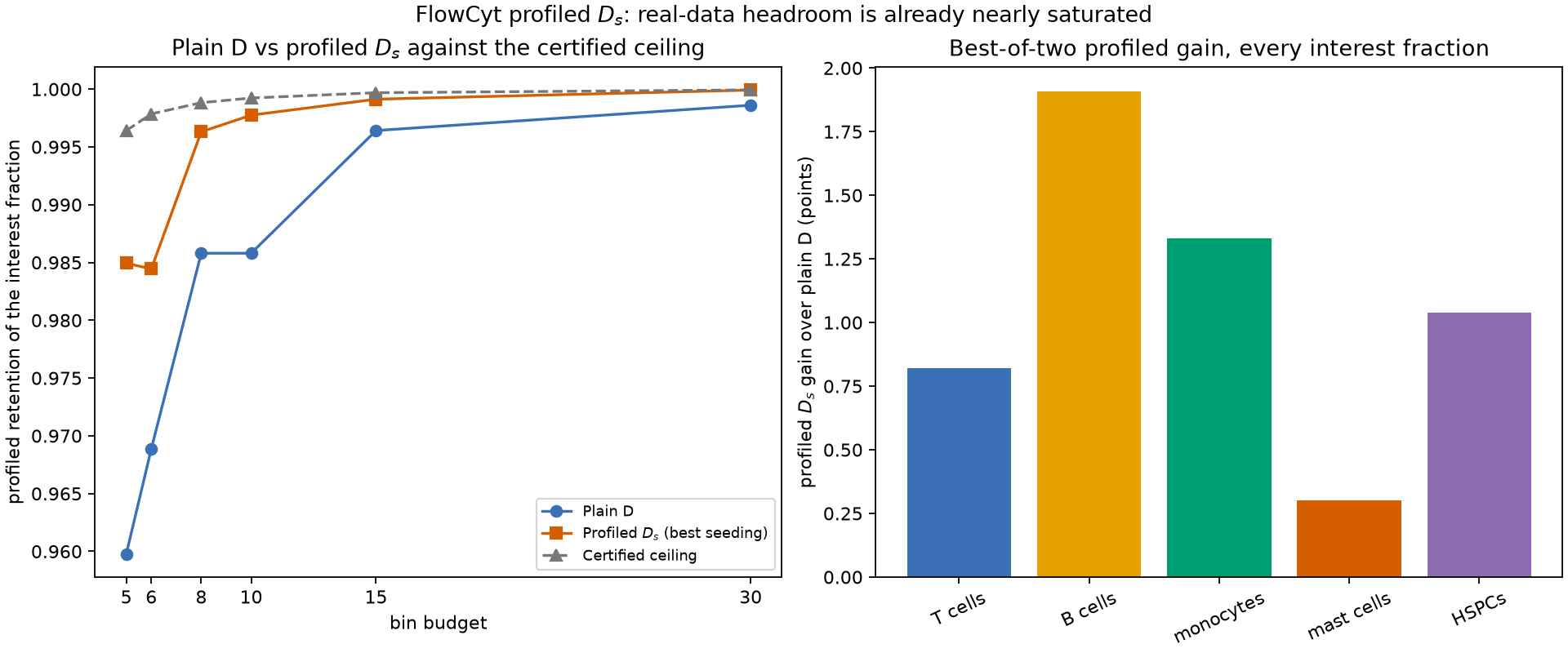
The left panel is the bin-budget sweep: plain D, the better of the two profiled seedings, and the certified ceiling, all against the bin budget on the 600,000-cell sample. The gap between the orange and grey lines is exactly the headroom table below quotes; it narrows from five bins to thirty. The right panel is the all-five-fractions sweep: the best-of-two profiled gain over plain D, in points, for every declared fraction of interest at the eight-bin operating point.

The nuisance parameterization is derived, not invented

Nothing here is a new model. The score page already established that the study's score matrix carries one column per free fraction of

\[ \theta=(\theta_{\mathrm T},\theta_{\mathrm B},\theta_{\text{mono}}, \theta_{\text{mast}},\theta_{\text{HSPC}}), \qquad \theta_{\text{other}}=1-\textstyle\sum_a\theta_a, \]

with

\[ s_a(x)=\frac{p_a(x)-p_{\text{other}}(x)}{\sum_k\theta_{0k}p_k(x)} =\frac{\partial}{\partial\theta_a}\log p(x\mid\theta)\bigg|_{\theta_0}. \]

So column \(a\) is the score of fraction \(a\), and the sixth component is already eliminated by the sum constraint. Declaring column \(a\) of interest and the remaining four columns nuisance therefore means exactly one thing: report \(\theta_a\) with the rest of the marrow composition floating. The Schur complement ProfiledDOptimality maximizes is the same Schur complement the downstream profile likelihood forms. No reparameterization, no invented calibration nuisance, no approximation.

Two consequences follow immediately, and both are constraints rather than choices.

• efficient_score_bound certifies a ceiling for one interest column, because a multivariate efficient score would need a multivariate D solver and the result would be a heuristic rather than a certificate. So the study declares one fraction at a time and sweeps all five.
• The headline fraction is fixed before any result is looked at. HSPCs are chosen on clinical grounds — the CD34+ compartment is the standard readout — and because their reference fraction, 0.00812, is far enough from zero that the downstream local covariance stays interpretable. Mast cells, at 0.00019, are the fraction the uncertainty audit already flags as boundary dominated. The full five-fraction sweep is published below so nobody has to take the choice on trust.

Two criteria, the same 27,607 rows

Both criteria see the same weighted score table: the 27,607-row partition subsample, weighted to reproduce \(\theta_0\) with equal patient influence inside each class. The bin budget is the study's operating point, eight.

interest = (4,)  # HSPCs
config = sq.DExchangeConfig(seed=2026, initializer_restarts=8)

plain = sq.optimize_partition(
    partition_scores,
    weights=partition_weights,
    n_bins=8,
    criterion=sq.DOptimality(),
    config=config,
)
bound = sq.efficient_score_bound(
    partition_scores,
    interest=interest,
    weights=partition_weights,
    n_bins=8,
    config=sq.ScalarDPConfig(seed=2026, max_rows=27_607),
)
profiled = sq.optimize_partition(
    partition_scores,
    weights=partition_weights,
    n_bins=8,
    criterion=sq.ProfiledDOptimality(interest),
    config=config,
    initial_labels=bound.labels,
)

All numbers in the tables below come from the 600,000-cell bounded sample unless a row says otherwise, and are asserted from flowcyt_profiled_ds.json at the end of this page.

Labeling	HSPC fraction alone	All five fractions	Relocations	Scans	Seconds
Plain D	0.98580	0.98705	0	1	1.7
Profiled \(D_s\), generic seeding	0.99631	0.03716	11,894	1,144	10.1
Profiled \(D_s\), ceiling-initialized	0.99618	0.00196	1,155	331	2.8
Certified ceiling	0.99883	—	—	—	18.0

Read the two retention columns against each other. Profiling gains 1.05 points of information about the HSPC fraction and gives up 95.0 points about the other four. That is not a defect of the optimizer; it is the criterion doing exactly what it was asked to do. The whole five-dimensional score space is collapsed onto the one efficient-score direction that carries HSPC information, and the rest of the geometry stops mattering.

Whether that trade is acceptable depends entirely on what will be written down. On FlowCyt it is not, for a reason the next two sections make precise.

The certified ceiling says there is almost nothing to win

efficient_score_bound builds the full-data efficient score \(\hat s=s_\psi-B^\ast s_\lambda\), partitions that one-dimensional coordinate exactly by weighted interval dynamic programming, and returns the resulting between-cell moment as a ceiling on the profiled objective of every eight-cell rule of the whole five-dimensional score space. It is a certificate, not an estimate.

At eight bins the ceiling is 0.99883. Plain D is already at 0.98580, so the entire headroom any criterion could ever recover is 1.30 points. The generically seeded profiled partition captures 80.7% of it and stops 0.00252 nats short of the ceiling; the ceiling-initialized run stops 0.00265 nats short.

That is the number that turns "profiling did not help much" into a statement. Without the certificate, a 1.05-point gain would be an invitation to tune the solver harder. With it, the remaining 0.25 points is provably all that is left, and it is worth less than the 95 points being spent to chase it.

The certificate is cheap relative to the study but not free: the exact scalar dynamic program is quadratic in the number of distinct efficient-score atoms, so on 27,607 rows it cost seconds rather than milliseconds. The budget sweep below records what it cost at each budget.

The bin budget, and where the initializer earns its place

Bins	Plain D	\(D_s\), generic seeding	\(D_s\), ceiling-initialized	Certified ceiling	Plain D, all five	\(D_s\), all five
5	0.95979	0.98494	0.98241	0.99642	0.10714	0.00076
6	0.96887	0.98445	0.98352	0.99786	0.98161	0.00031
8	0.98580	0.99631	0.99618	0.99883	0.98705	0.00196
10	0.98580	0.99701	0.99775	0.99923	0.99190	0.00774
15	0.99642	0.99708	0.99913	0.99969	0.99635	0.00413
30	0.99861	0.99941	0.99992	0.99993	0.99908	0.01008

Taking the better of the two profiled runs at each budget, the gain over plain D is 2.51 points at five bins, 1.56 at six, 1.05 at eight, 1.19 at ten, 0.27 at fifteen, and 0.13 at thirty. It is not monotone — both sides are local searches, and eight bins happens to be a good budget for plain D and ten a slightly worse one — but the direction is unambiguous, and so is the reason: the certified headroom itself shrinks from 3.66 points at five bins to 0.13 at thirty, and by thirty bins the profiled run has taken 99% of everything that was ever there.

Two caveats belong with this table rather than after it. The five-bin row is below the identifiability threshold, so its 2.51-point gain is a gain in a quantity the patient likelihood cannot use — the next section makes that precise. And the last two columns do not shrink at all: the profiled partition is catastrophic for the other four fractions at every single budget.

The ceiling's own interval labels are also an initializer, and what they buy splits cleanly in two:

Bins	Certified gap, generic	Certified gap, initialized	Relocations, generic	Relocations, initialized	Scans, generic	Scans, initialized
5	0.011588	0.014155	28,537	394	3,483	73
6	0.013533	0.014478	14,521	506	2,653	224
8	0.002524	0.002652	11,894	1,155	1,144	331
10	0.002229	0.001485	10,610	799	177	425
15	0.002616	0.000562	650	709	30	383
30	0.000527	0.000015	408	1,295	56	470

At small budgets the initializer buys cost: at five bins, 394 accepted relocations instead of 28,537, and 73 scans instead of 3,483, for a slightly worse optimum. At ten bins and above it buys quality: at thirty bins it closes the certified gap by a factor of 34.

Neither effect is a guarantee, and the table says so plainly in both directions. Supplied labels replace the seeding of the first restart only, so the other restarts still explore — and at five, six, and eight bins one of those generic restarts lands slightly higher than the ceiling's own labels do. Profiled exchange is a local search; starting it inside the geometry of the relaxed problem it is trying to beat is a good heuristic, not a theorem, and the certificate is what makes the difference legible.

Wall clock is machine dependent, but its shape is not: the exact scalar dynamic program is quadratic in the number of distinct efficient-score atoms, so on 27,607 rows it cost roughly 16 seconds at eight bins and 58 at thirty on the machine that produced this evidence.

What the fixed-total likelihood actually sees

profiled_information_report follows the library's uncentered intensity convention. The FlowCyt patient fit conditions on 20,000 cells, so it sees the fixed-total information instead — the same subtraction of the global mean score that makes five bins fail for the joint fit. Profiling does not change that, and the two conventions do not always agree.

Bins	\(D_s\) profiled retention (intensity)	Plain D, fixed total	\(D_s\), fixed total	Retained fixed-total rank
5	0.98241	0.00000	0.00000	4
6	0.98352	0.96887	0.96854	5
8	0.99618	0.98580	0.99618	5
30	0.99992	0.99861	0.99992	5

Two things worth stating out loud.

At five bins the intensity-convention column reads 0.98241 while the quantity the measurement depends on is exactly zero. Profiling changes what you optimize, not what you can identify: with only four independent bin frequencies, no amount of nuisance projection makes the HSPC fraction estimable while the other four fractions float. That is the same wall the joint fit hits, arriving from a different direction.

At six bins the criterion improves the intensity-convention profiled retention from 0.96887 to 0.98352 and, in the fixed-total convention that matters, moves it from 0.96887 to 0.96854 — very slightly down, while its all-five retention collapses to 0.00031. Six bins is a budget at which profiled \(D_s\) is strictly harmful on this problem. From eight bins upward the two conventions agree to five decimals, and the criterion's gain is real but small.

The rule you could actually deploy

Everything above labels one fixed sample. PartitionResult has no predict_scores, on purpose. An exchange-stable plain-D partition compiles — Chapter 8's Theorem 3 guarantees its labels are the training realization of a Mahalanobis nearest-cell rule. A profiled partition has no such guarantee, and Chapter 10 exhibits a finite table whose globally optimal profiled labeling violates the geometry it induces, so the library refuses to invent one. A reusable profiled rule has to be fitted as one, which SoftVoronoiConfig does.

Rule	Held out, HSPC alone	Held out, all five	Occupied bins	HSPC RMSE	Mean 68% half-width	Seconds
Plain D, compiled exchange	0.98782	0.98528	8	0.002751	0.000882	0.6
Profiled \(D_s\), soft Voronoi	0.98665	0.97186	8	0.002340	0.000885	0.9

This is the table the page exists for, and it reports a flat result.

The half-width is the number the measurement would quote: the local 68% interval for the HSPC fraction with the other five floating, averaged over the ten held-out patients. The profiled rule's interval is 0.33% wider, not narrower. Its realized HSPC RMSE is lower by \(4.1\times10^{-4}\), but ten patients cannot resolve a difference that small, and the RMSE is a property of the re-estimated template model rather than of the score-space objective — the two are different quantities, exactly as the unbinned-baseline discussion explains.

The reason the deployable rule shows none of the free-label partition's 1.05-point gain is structural: the soft profiled fit is restricted to nearest-center cells, and inside that family the profiled optimum is essentially the plain-D optimum. Its held-out all-five retention drops by 1.34 points for nothing. The free-label profiled partition that does capture the gain is not a rule and never will be.

Note that the held-out columns use the empirical test measure — one unit of weight per cell — while the training columns use the \(\theta_0\) integration measure. They are different measures, which is why a held-out number can exceed its training counterpart without anything being wrong.

All five fractions

The comparison does not depend on the fraction chosen. Plain D is the same partition in every row; only the declared interest column changes.

Interest fraction	\(\theta_0\)	Plain D	\(D_s\), generic	\(D_s\), initialized	Ceiling	Gain	\(D_s\), all five
T cells	0.07113	0.99044	0.99889	0.99865	0.99958	+0.00821	0.00511
B cells	0.01959	0.97842	0.99812	0.99752	0.99920	+0.01910	0.00690
Monocytes	0.01498	0.98479	0.99844	0.99811	0.99949	+0.01332	0.00216
Mast cells	0.00019	0.99600	0.99881	0.99902	0.99989	+0.00303	0.00002
HSPCs	0.00812	0.98580	0.99631	0.99618	0.99883	+0.01038	0.00196

Every fraction tells the same story with different numbers. The largest gain is B cells at 1.9 points, and even there plain D starts within 2.1 points of a ceiling it cannot exceed, and the profiled partition pays 98 points of all-five retention for the improvement. No fraction is an exception.

Does it hold at CI scale?

The frozen 34,554-cell fixture runs the same study in about 100 seconds and reproduces every qualitative conclusion, with the caveat the data page states: the fixture is class-balanced, so its reference composition is near-uniform and its absolute retentions are higher throughout.

Quantity, HSPCs at 8 bins	Frozen CI fixture (34,554 cells)	Bounded sample (600,000 cells)
Plain D, profiled retention	0.99539	0.98580
\(D_s\) best of two seedings	0.99924	0.99631
Certified ceiling	0.99967	0.99883
Profiled gain	+0.00385	+0.01051
All-five retention given up	0.87705	0.94989
Half-width ratio, \(D_s\) rule over D rule	1.0177	1.0033

Both scales agree that the profiled criterion improves its own objective, that the improvement is bounded by a certificate that is already nearly saturated, that the cost in all-five retention is severe, and that the deployable profiled rule's downstream interval is wider rather than narrower.

Every number on this page

import json
from pathlib import Path

evidence = json.loads(Path("docs/usecases/assets/flowcyt_profiled_ds.json").read_text())
sample, fixture = evidence["sample_scale"], evidence["fixture_scale"]

# Provenance: the two scales, and the digest of the bounded sample.
assert sample["run"]["provenance"]["scale"] == "600,000-cell bounded sample"
assert sample["run"]["rows"]["total"] == 600_000
assert sample["run"]["rows"]["partition"] == 27_607
assert (
    sample["run"]["provenance"]["sample_sha256"]
    == "a08e9bf183fe32b913e155d413eeacfdb65c7f99017a42e69c4b91bdde20d987"
)
assert fixture["run"]["provenance"]["scale"] == "frozen CI fixture"
assert fixture["run"]["rows"]["total"] == 34_554

# The declared nuisance parameterization.
assert sample["interest_index"] == 4
assert sample["interest_population"] == "HSPCs"
assert sample["nuisance_populations"] == ["T cells", "B cells", "monocytes", "mast cells"]
assert sample["reference_component"] == "other"
assert round(sample["reference_composition"][4], 5) == 0.00812

partitions = {row["key"]: row for row in sample["partitions"]}
plain = partitions["d_partition"]
seeded = partitions["ds_partition_seeded"]
initialized = partitions["ds_partition_initialized"]

assert round(plain["profiled_retention"], 5) == 0.98580
assert round(plain["full_retention"], 5) == 0.98705
assert plain["accepted_moves"] == 0 and plain["scans"] == 1
assert round(seeded["profiled_retention"], 5) == 0.99631
assert round(seeded["full_retention"], 5) == 0.03716
assert seeded["accepted_moves"] == 11_894 and seeded["scans"] == 1_144
assert round(initialized["profiled_retention"], 5) == 0.99618
assert round(initialized["full_retention"], 5) == 0.00196
assert initialized["accepted_moves"] == 1_155 and initialized["scans"] == 331

# The trade, and the certified headroom it lives inside.
gain = seeded["profiled_retention"] - plain["profiled_retention"]
given_up = plain["full_retention"] - seeded["full_retention"]
headroom = sample["bound"]["ceiling_retention"] - plain["profiled_retention"]
assert round(gain, 5) == 0.01051
assert round(given_up, 5) == 0.94989
assert round(sample["bound"]["ceiling_retention"], 5) == 0.99883
assert round(headroom, 5) == 0.01303
assert round(gain / headroom, 3) == 0.807
assert round(sample["bound"]["seeded_gap"], 6) == 0.002524
assert round(sample["bound"]["initialized_gap"], 6) == 0.002652

# The bin-budget sweep, including the fixed-total convention.
budgets = {row["n_bins"]: row for row in sample["budget_sweep"]}
assert sorted(budgets) == [5, 6, 8, 10, 15, 30]
for n_bins, row in budgets.items():
    assert row["d_profiled_retention"] <= row["ceiling_retention"] + 1e-9
    assert row["ds_initialized_retention"] <= row["ceiling_retention"] + 1e-9

five = budgets[5]
assert five["fixed_total_rank_d"] == 4 and five["fixed_total_rank_ds"] == 4
assert five["d_fixed_total_retention"] == 0.0
assert five["ds_initialized_fixed_total_retention"] == 0.0
assert round(five["ds_initialized_retention"], 5) == 0.98241

six = budgets[6]
assert six["fixed_total_rank_ds"] == 5
assert round(six["d_fixed_total_retention"], 5) == 0.96887
assert round(six["ds_initialized_fixed_total_retention"], 5) == 0.96854
assert six["ds_initialized_fixed_total_retention"] < six["d_fixed_total_retention"]
assert round(six["ds_initialized_full_retention"], 5) == 0.00031

best_gain = {
    n_bins: max(row["ds_seeded_retention"], row["ds_initialized_retention"])
    - row["d_profiled_retention"]
    for n_bins, row in budgets.items()
}
assert [round(100 * best_gain[n], 2) for n in (5, 6, 8, 10, 15, 30)] == [
    2.51,
    1.56,
    1.05,
    1.19,
    0.27,
    0.13,
]
headroom_by_bins = {
    n_bins: row["ceiling_retention"] - row["d_profiled_retention"]
    for n_bins, row in budgets.items()
}
assert round(100 * headroom_by_bins[5], 2) == 3.66
assert round(100 * headroom_by_bins[30], 2) == 0.13
assert round(best_gain[30] / headroom_by_bins[30], 2) == 0.99

assert round(budgets[30]["initialized_gap"], 6) == 0.000015
assert round(budgets[30]["seeded_gap"] / budgets[30]["initialized_gap"]) == 34
assert budgets[5]["seeded_moves"] == 28_537 and budgets[5]["initialized_moves"] == 394
# Wall clock is machine dependent; only its order of magnitude is published.
assert 5.0 < budgets[8]["bound_seconds"] < 40.0
assert budgets[30]["bound_seconds"] > budgets[8]["bound_seconds"]

# The deployable rules and the interval they imply.
rules = {row["key"]: row for row in sample["rules"]}
d_rule, ds_rule = rules["d_rule"], rules["ds_rule"]
assert d_rule["solver"] == "DExchangeConfig" and ds_rule["solver"] == "SoftVoronoiConfig"
assert round(d_rule["test_profiled_retention"], 5) == 0.98782
assert round(ds_rule["test_profiled_retention"], 5) == 0.98665
assert round(d_rule["test_full_retention"], 5) == 0.98528
assert round(ds_rule["test_full_retention"], 5) == 0.97186
assert d_rule["test_occupied_bins"] == ds_rule["test_occupied_bins"] == 8
assert round(d_rule["downstream"]["interest_rmse"], 6) == 0.002751
assert round(ds_rule["downstream"]["interest_rmse"], 6) == 0.002340
assert round(d_rule["downstream"]["mean_half_width"], 6) == 0.000882
assert round(ds_rule["downstream"]["mean_half_width"], 6) == 0.000885
# The profiled rule's reported interval is wider, not narrower.
half_width_ratio = (
    ds_rule["downstream"]["mean_half_width"] / d_rule["downstream"]["mean_half_width"]
)
assert round(half_width_ratio, 4) == 1.0033
assert ds_rule["downstream"]["converged_patients"] == 10

# Every fraction, not just the declared one.
sweep = {row["population"]: row for row in sample["interest_sweep"]}
assert list(sweep) == ["T cells", "B cells", "monocytes", "mast cells", "HSPCs"]
assert round(sweep["B cells"]["gain"], 5) == 0.01910
assert max(round(row["gain"], 5) for row in sweep.values()) == 0.01910
for row in sweep.values():
    assert row["ds_initialized_retention"] <= row["ceiling_retention"] + 1e-9
    assert row["ds_full_retention"] < 0.01

# The fixture-scale replication.
fixture_partitions = {row["key"]: row for row in fixture["partitions"]}
fixture_rules = {row["key"]: row for row in fixture["rules"]}
assert round(fixture_partitions["d_partition"]["profiled_retention"], 5) == 0.99539
assert round(fixture_partitions["ds_partition_seeded"]["profiled_retention"], 5) == 0.99924
assert round(fixture["bound"]["ceiling_retention"], 5) == 0.99967
fixture_ratio = (
    fixture_rules["ds_rule"]["downstream"]["mean_half_width"]
    / fixture_rules["d_rule"]["downstream"]["mean_half_width"]
)
assert round(fixture_ratio, 4) == 1.0177
assert fixture_ratio > 1.0 and half_width_ratio > 1.0

What this establishes, and what it does not

Task and door. Sample partitioning is the main event — optimize_partition under both criteria — with space quantization brought in through fit_quantizer to supply the held-out and downstream columns. The door is unchanged from the rest of the study: Door 3, a trained classifier converted to mixture scores.

Criteria and solvers. DOptimality and ProfiledDOptimality with the exact positive-gain exchange, the exact scalar dynamic program inside efficient_score_bound, and SoftVoronoiConfig for the reusable profiled rule — every pairing one the dispatch table declares.

The result. On FlowCyt, at the study's operating point, ProfiledDOptimality should not be used. That conclusion is supported rather than asserted: the certified ceiling bounds the total available gain at 1.30 points, the free-label profiled partition recovers 80.7% of it while destroying 95 points of everything else, and the only deployable profiled object — the soft rule — reports an interval 0.33% wider than plain D's. Recommending against a feature on measured evidence is a use of the feature, not an argument against having it.

The honest caveats.

• Every retention here is retention of the supplied score law, with information_kind equal to supplied_score_surrogate. The score page explains why that is a bounded claim, and it bounds this page's claims too.
• The downstream half-widths come from re-estimated templates and a fixed-total multinomial likelihood, not from the score-space Fisher matrix. They are the right quantity to compare, and they are not the quantity either criterion optimizes.
• Ten held-out patients cannot resolve RMSE differences of order \(10^{-4}\). The interval widths, which are computed rather than sampled, are the load-bearing comparison.
• The certified ceiling applies to eight-cell rules of this weighted score table. It transfers to a different sample, a different weighting, or a different bin budget only by being recomputed, which is why the sweep recomputes it at every budget.
• There is no compile bridge for \(D_s\) and there will not be one. The finite profiled optimum is not forced into the geometry it induces; the exact rational counterexample is ds-geometry-counterexample.

Reproduce

The study honors SCOREQUANT_EXAMPLE_FAST and runs at either scale. The fixture-scale run takes about 100 seconds end to end:

JAX_ENABLE_X64=1 MPLBACKEND=Agg \
  uv run python -m examples.cell_population \
  --profiled --quick \
  --fixture examples/data/flowcyt_fixture.npz

The bounded-sample run splits into a preparation stage and the study itself, so a long run resumes from the cached score table instead of refitting the classifier:

JAX_ENABLE_X64=1 MPLBACKEND=Agg \
  uv run python -m examples.cell_population \
  --profiled-prepare-only --full \
  --fixture flowcyt-results/flowcyt_sample_20000.npz \
  --profiled-cache flowcyt-results/profiled_inputs_sample.npz

JAX_ENABLE_X64=1 MPLBACKEND=Agg \
  uv run python -m examples.cell_population \
  --profiled --full \
  --fixture flowcyt-results/flowcyt_sample_20000.npz \
  --profiled-cache flowcyt-results/profiled_inputs_sample.npz

Preparation took 139 seconds and the study 432 seconds for the published run. Both commands merge their scale into flowcyt_profiled_ds.json without disturbing the other.