Door 1: precomputed score events

This page walks both public tasks — sample partitioning (optimize_partition) and space quantization (fit_quantizer) — through Door 1: you already have (event, score) rows and their weights, so no provider is needed. It replaces the old "first analytic partition" tutorial and answers a question that comes up immediately: once you have a stable partition of your sample, when do you compile it into a rule, and when do you just fit a rule directly?

Problem

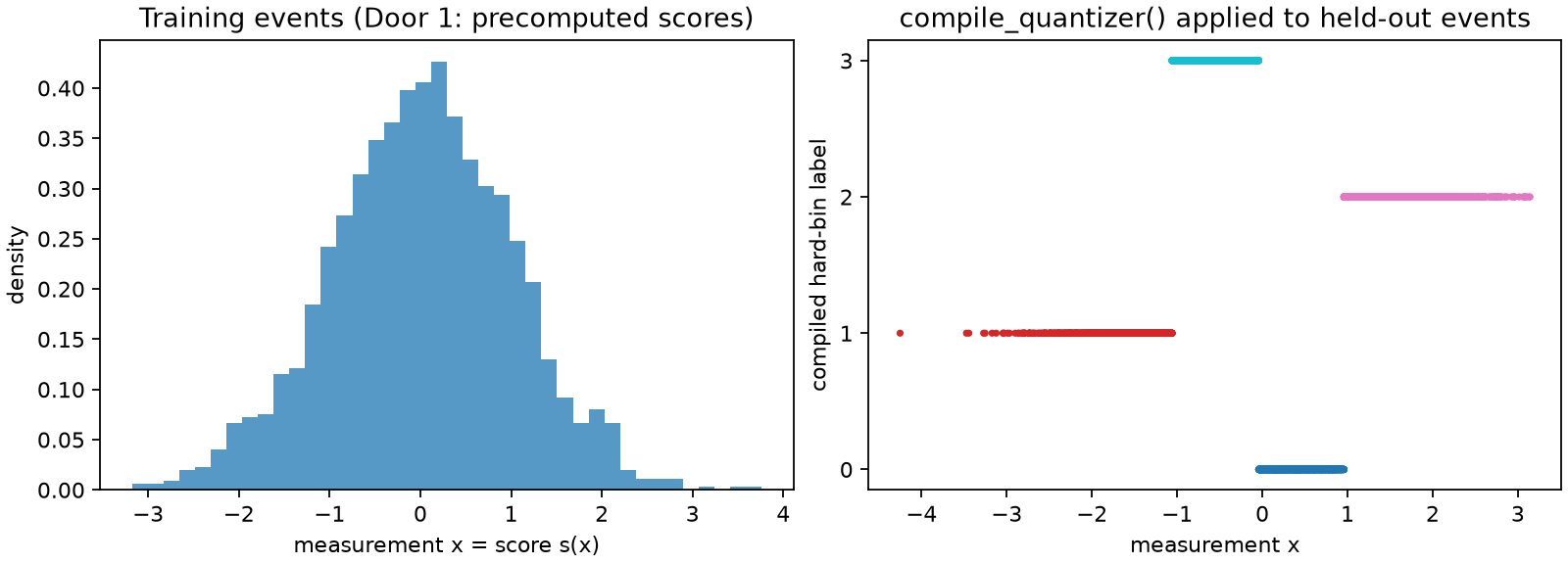
Each event is one measurement \(x\sim\mathcal N(\mu,1)\), and the downstream task is to estimate the unknown location \(\mu\). At the reference point \(\mu_0=0\), the score is \(s(x)=x\), so the observation and its score coincide — a useful analytic check, since grouping nearby score values should preserve information about \(\mu\) and the amount lost can be measured exactly.

Data

examples.synthetic_problems.gaussian_location returns deterministic train/validation/test splits of this model. The scores are declared exact at the reference point, so information_kind is later allowed to read "exact_fisher".

import numpy as np

import scorequant as sq
from examples.synthetic_problems import gaussian_location

problem = gaussian_location()
train, test = problem.train, problem.test

provenance = sq.ScoreProvenance(kind="exact", reference_point=(0.0,))
sample = sq.ScoreSample(train.scores, train.weights, provenance=provenance)
assert sample.scores.shape == (2000, 1)

API walkthrough

optimize_partition, with a stability report

optimize_partition assigns labels to exactly the 2000 rows supplied. exchange_stable and best_remaining_gain are that assignment's own certificate: they report whether any single admissible relocation could still improve the exact objective.

partition = sq.optimize_partition(
    sample.scores,
    weights=sample.weights,
    n_bins=4,
    criterion=sq.DOptimality(),
    config=sq.DExchangeConfig(seed=12),
    provenance=sample.provenance,
)
assert partition.exchange_stable is True
assert partition.best_remaining_gain < 0.0  # no move would raise the objective
train_efficiency = float(partition.train_report.geometric_mean_retention)
assert 0.85 < train_efficiency < 0.92

The same certificate is checkable independently of how the labels were produced, through exchange_stability_report:

stability = sq.exchange_stability_report(
    partition.training_scores, partition.labels, weights=sample.weights
)
assert stability.stable == partition.exchange_stable

partition.labels belongs to these 2000 rows and nothing else — PartitionResult has no predict_scores.

The compile bridge

Because the partition is exchange-stable and the criterion is DOptimality, it is already a strict self-consistent Voronoi partition in the retained Mahalanobis metric (Chapter 6 proves why). compile_quantizer() turns that fact into a QuantizerResult and verifies it reproduces every training label before returning:

compiled = partition.compile_quantizer()
compiled_test = compiled.evaluate_scores(test.scores, test.weights)
compiled_retention = float(compiled_test.geometric_mean_retention)
assert 0.85 < compiled_retention < 0.92
future_bins = compiled.predict_scores(np.array([[0.4], [-1.2]]))

fit_quantizer directly, as the alternative

If a reusable rule is the goal from the start, fit one directly instead of routing through a partition. This also opens criteria and solvers compile_quantizer cannot reach — here, normalized-trace k-means instead of D-optimal exchange:

direct = sq.fit_quantizer(
    sample,
    n_bins=4,
    criterion=sq.NormalizedTrace(),
    config=sq.KMeansConfig(seed=12, solver_restarts=4),
)
direct_retention = float(direct.evaluate_scores(test.scores, test.weights).geometric_mean_retention)
assert 0.85 < direct_retention < 0.92
assert round(compiled_retention, 6) == round(direct_retention, 6)

On this one-dimensional problem the two routes land on the same test-set D-efficiency to six decimal places — both are approximating the same optimal interval partition. That agreement is a property of this simple problem, not a guarantee; a later solver-shootout page compares every solver against every baseline on a harder, two-parameter problem where they separate.

Analysis

Route	Criterion / solver	Certificate	Reusable?
optimize_partition alone	any	exchange_stable, best_remaining_gain	no — PartitionResult has no predict method
optimize_partition → compile_quantizer()	DOptimality only, exchange-stable, nonsingular	Theorem-backed Mahalanobis rule	yes
fit_quantizer directly	DOptimality, ProfiledDOptimality, or NormalizedTrace, any solver	the fit's own diagnostics	yes

Discussion

Task: both — sample partitioning first, then either the compile bridge or a direct fit into space quantization. Door: 1, precomputed (event, score) rows via ScoreSample. Criterion / solver: DOptimality with exact exchange for the partition and its compiled rule; NormalizedTrace with k-means for the direct alternative.

Use optimize_partition → compile_quantizer() when you specifically want the D-optimal exchange result and its exchange-stability certificate, and only need a reusable rule as a by-product of a result you were already computing. Use fit_quantizer directly when you know from the start you want a rule, or when you want a criterion or solver the compile bridge does not reach — NormalizedTrace, ProfiledDOptimality, or the soft-Voronoi and scalar dynamic-programming solvers all skip the partition step entirely. See Chapter 4 for where scores and doors come from, and Chapter 6 for the theorem behind the compile bridge.

The matching notebook, door1_score_events.ipynb, runs the fuller study with more restarts and a closer look at where the two routes would disagree on a harder problem.