4. Scores, score laws, and the three doors

The first three chapters treated the score as if it were simply the data. For the Gaussian location model that was literally true — \(s(x)=x\) — which is why the arithmetic stayed transparent. This chapter pays that debt. What is a score, why is it the right thing to bin, and where does one actually come from when the model is not a textbook Gaussian?

What the score is

Fix a model \(p(x\mid\theta)\) and a reference point \(\theta_0\). Expanding the log likelihood of one event around that point,

\[\log p(x\mid\theta) \;=\; \log p(x\mid\theta_0) \;+\; s(x)^\top(\theta-\theta_0) \;+\; O\big(\|\theta-\theta_0\|^2\big), \qquad s(x) = \nabla_\theta \log p(x\mid\theta)\big|_{\theta_0},\]

so the score is the event's local opinion about \(\theta\): a vector in parameter space whose direction says which parameter combinations the event favors and whose length says how strongly. Two events with the same score are locally indistinguishable as evidence, however different they look in the detector. Summing the outer products over the reference measure gives the Fisher information \(I_{\text{full}} = \mathbb{E}\big[s(X)s(X)^\top\big]\).

The score has units, an origin, and an orientation, all of which are statistical rather than conventional. Replacing \(s\) by \(As\) with \(A\) invertible is a reparameterization of \(\theta\), and criteria such as the log determinant are designed to be invariant under it. Replacing \(s\) by \(s - c\) is not a reparameterization: it is a different statistical problem. For a normalized probability model the score happens to have mean zero, so shifting looks harmless; for a Poisson intensity model \(\lambda(x;\theta)\) the event score \(s_\alpha(x) = \partial_{\theta_\alpha}\log\lambda\) has a nonzero mean under the intensity measure, and subtracting it deletes the total-rate direction — a real parameter, silently discarded. This is why nothing in ScoreQuant ever centers a score table, and why the origin of score space is protected throughout the book.

The score law is the whole input

Let \(q:\mathbb{R}^d\to\{1,\dots,K\}\) be a hard rule on score space, so that the observation-space compressor is \(Q(x) = q(s(x))\). Every quantity the criteria of this book depend on is a cell probability or a cell score moment,

\[W_b = \Pr\big(q(S)=b\big), \qquad m_b = \mathbb{E}\big[S\,\mathbf{1}\{q(S)=b\}\big],\]

and both are integrals of functions of \(S\) alone. They therefore depend on the observation model only through the push-forward score law

\[P_S \;=\; s_{\#}P_{\theta_0},\]

the distribution of \(S\) when \(X\sim P_{\theta_0}\). Two entirely different experiments with the same score law pose the same binning problem and have the same optimal rules. This is a genuine simplification: it removes the observation space, whatever its dimension and structure, from every algorithm in this book.

It is also not a new observation. Quantizing the score to preserve Fisher information was posed directly for distributed estimation by Venkitasubramaniam, Tong and Swami (2006). Barnes, Han and Özgür (2018) characterized the Fisher information of a quantized observation geometrically through conditional score means — the identity Chapter 5 uses throughout — and solved the one-bit Gaussian location problem exactly, recovering the half-space rule of Chapter 2. Dülek (2023) proved for exponential families that an optimal \(K\)-level quantizer can be taken to depend only on the sufficient statistic and that the trace-optimal partition is convex-polytopal, so polyhedral quantizer geometry is established prior art rather than a contribution. The detection-side analogue is older still: Tsitsiklis (1993) established the corresponding sufficiency of likelihood-ratio space for quantizer design in hypothesis testing. What this book adds begins in Chapter 8 and concerns the exact finite structure of the full-matrix determinant criterion, not the choice of score space.

Two contracts, not one

A score law is a map plus a measure. Knowing \(s(x)\) for every \(x\) tells you where each event lands in score space; it says nothing about how many events land where. So ScoreQuant separates the two:

Contract	Supplies	Examples
Source	the reference measure — which events exist, with what weight	ScoreSample, ObservationSample, IntegrationSource
Score provider	the observation-to-score map	ScoreFunction, LinearComponentScore, DensityRatioScore, CentralLogRatioScore

The pairing is validated rather than guessed. A ScoreSample is already in score space, so it rejects a provider; an ObservationSample or IntegrationSource is in observation space, so it requires one. A score callback offered on its own is refused, because automatic differentiation and trained classifiers supply the map and never the measure.

There is a matching split on the output side, which Chapter 6 develops in full: optimize_partition labels one fixed table and returns no predictor, while fit_quantizer learns a reusable rule whose only prediction method is predict_scores. Converting observations to scores stays a line you wrote, visible in your own code.

Door 1: the scores already exist

The simplest case. Somebody — you, a colleague, a simulator's weight-derivative output — has already produced a score column.

import math

import numpy as np

import scorequant as sq

rng = np.random.default_rng(4)
observations = rng.normal(size=(4_000, 1))  # X ~ N(theta, 1) at theta0 = 0
precomputed = np.asarray(observations)  # so the score is s(x) = x

door1 = sq.ScoreSample(
    precomputed,
    provenance=sq.ScoreProvenance(kind="exact", reference_point=(0.0,)),
)
quantizer = sq.fit_quantizer(
    door1, n_bins=4, criterion=sq.DOptimality(), config=sq.ScalarDPConfig()
)
partition = sq.optimize_partition(precomputed, n_bins=4, config=sq.DExchangeConfig(seed=4))

assert quantizer.information_kind == "exact_fisher"
assert hasattr(quantizer, "predict_scores")
assert not hasattr(partition, "predict_scores")

ScoreProvenance is how you declare where the numbers came from. Only "exact" and "autodiff" let a result describe its matrices as Fisher information; everything else reports "supplied_score_surrogate", for reasons the last section of this chapter makes concrete.

Door 2: a model you can differentiate

When an analytic likelihood or intensity is available, the score is a function you can write down or differentiate automatically. ScoreFunction wraps any callable [N, D] -> [N, P], and LinearComponentScore evaluates a linear component model, for which \(\lambda(x;\theta)=\sum_\alpha \theta_\alpha\phi_\alpha(x)\) gives \(s_\alpha = \phi_\alpha/\lambda\) directly.

exact_score = sq.ScoreFunction(
    lambda X: np.asarray(X),
    provenance=sq.ScoreProvenance(kind="exact", reference_point=(0.0,)),
)
door2 = sq.fit_quantizer(
    sq.ObservationSample(observations),
    provider=exact_score,
    n_bins=4,
    criterion=sq.DOptimality(),
    config=sq.ScalarDPConfig(),
)

# Same events, same map, therefore the same score law and the same answer.
assert np.array_equal(np.asarray(door2.labels), np.asarray(quantizer.labels))

A sample is not the only way to carry a measure. For a bounded low-dimensional model the reference measure can be supplied deterministically, as an explicit density on a box evaluated at Gauss-Legendre nodes. There is no sampling noise in the result at all.

population = sq.IntegrationSource(
    [[-8.0, 8.0]],
    density=lambda X: np.exp(-0.5 * np.asarray(X)[:, 0] ** 2) / math.sqrt(2.0 * math.pi),
    quadrature=sq.GaussLegendreConfig(order=200),
)
door2_population = sq.fit_quantizer(
    population,
    provider=exact_score,
    n_bins=4,
    criterion=sq.DOptimality(),
    config=sq.ScalarDPConfig(),
)

# Chapter 2 computed the four-cell population optimum in closed form.
assert abs(float(door2_population.train_report.geometric_mean_retention) - 0.882518) < 0.02

Bounds alone never imply a uniform measure — the density is mandatory — and the node count is order ** D, so this door closes quickly above a few dimensions. Beyond that, use a sample.

Door 3: estimated density ratios

Often there is no evaluable likelihood at all: the model is a simulator, the detector response is learned, the background is data. The score can still be estimated. Generate samples at \(\theta_0-\delta_j e_j\) and \(\theta_0+\delta_j e_j\) and train a calibrated binary classifier \(D_j\) to tell them apart. With equal training priors the Bayes-optimal logit is the log likelihood ratio — the observation that Cranmer, Pavez and Louppe (2015) turned into a practical method — so

\[\operatorname{logit} D_j(x) = \log\frac{p(x\mid\theta_0+\delta_j e_j)}{p(x\mid\theta_0-\delta_j e_j)}, \qquad \hat s_j(x) = \frac{1}{2\delta_j}\operatorname{logit} D_j(x)\]

is a central finite-difference estimate of the \(j\)-th score coordinate, with deterministic bias \(O(\delta_j^2)\). Using the local score as the learned summary of a simulator is the SALLY/SALLINO construction of Brehmer, Louppe, Pavez and Cranmer (2020). If the priors of the two training samples are unequal, their log-odds must be subtracted from the logit before dividing.

ScoreQuant begins at the trained model. Training, cross-fitting and calibration stay in your application; the library takes a ready probability callback and applies the pure prior-corrected transform.

delta = 0.5


def calibrated(X):
    """Bayes-optimal minus/plus probabilities for N(-delta, 1) against N(+delta, 1)."""
    plus = 1.0 / (1.0 + np.exp(-2.0 * delta * np.asarray(X)[:, 0]))
    return np.stack([1.0 - plus, plus], axis=1)


door3 = sq.CentralLogRatioScore(calibrated, [delta], [0.5, 0.5])
recovered = np.asarray(door3.score(observations))[:, 0]

assert np.max(np.abs(recovered - observations[:, 0])) < 1e-5
assert door3.provenance.kind == "estimated_ratio"

Here the classifier is the exact Bayes rule and the Gaussian location model is exponential in \(x\), so the finite-difference construction recovers \(s(x)=x\) to the working precision of the arithmetic, for any \(\delta\). Running that check against your own callback, on a model where you know the answer, is the cheapest calibration diagnostic there is.

For a finite mixture whose parameters are the component fractions the ratio is the representation itself. A calibrated multiclass classifier estimates posteriors \(\eta_\alpha(x)\propto \pi_\alpha \phi_\alpha(x)\); dividing by the known training priors (ratios_from_posteriors) recovers the component density ratios, and mixture_scores_from_ratios applies the simplex-constrained algebra that turns them into scores — DensityRatioScore.from_classifier packages the chain as a provider. The same provider accepts a ratio callback from any other backend: an analytic formula, a direct density-ratio estimator, a calibrated neural likelihood-ratio model. The three-doors guide works through the constructions with the exact shape and normalization requirements.

Estimated scores are not Fisher information

Door 3 buys reach at a price, and the price deserves to be stated bluntly. The between-cell algebra is exact for whatever vectors you supply. If those vectors are \(\hat s \ne s\), the matrix a report contains is \(\operatorname{Var}\big(\mathbb{E}[\hat s\mid q(\hat s)]\big)\) — a surrogate — while the information the labels actually retain about \(\theta\) is \(\operatorname{Var}\big(\mathbb{E}[s\mid q(\hat s)]\big)\). The two coincide only when the estimated score is the true one.

The gap is not academic. Suppose the two training samples behind the classifier were imbalanced, 40/60 rather than 50/50, and that imbalance was never declared. The transform then subtracts the wrong log-odds and returns \(\hat s(x) = x + c\) with \(c = \log(1.5)/(2\delta)\). Watch what that does to the two numbers.

def imbalanced(X):
    """The same classifier, trained with 40/60 priors that were never declared."""
    odds = np.exp(2.0 * delta * np.asarray(X)[:, 0]) * (0.6 / 0.4)
    plus = odds / (1.0 + odds)
    return np.stack([1.0 - plus, plus], axis=1)


misdeclared = sq.CentralLogRatioScore(imbalanced, [delta], [0.5, 0.5])
offset = np.asarray(misdeclared.score(observations))[:, 0] - observations[:, 0]
assert abs(float(offset.mean()) - math.log(1.5) / (2 * delta)) < 1e-5

biased = sq.fit_quantizer(
    sq.ScoreSample(np.asarray(misdeclared.score(observations))),
    n_bins=2,
    criterion=sq.DOptimality(),
    config=sq.ScalarDPConfig(),
)
reported = float(biased.train_report.geometric_mean_retention)
true = float(sq.information_report(observations, biased.labels, n_bins=2).geometric_mean_retention)

assert reported > true + 0.03  # the surrogate number is inflated
assert abs(true - 2.0 / math.pi) < 0.02  # the information actually kept is unchanged
assert biased.information_kind == "supplied_score_surrogate"
print(round(reported, 5), round(true, 5))

The misdeclared classifier reports 0.687 where the honest answer is 0.635. It looks better than the correctly declared one, and it is not. The mechanism is worth following. Retention is the ratio \(I_q/I_{\text{full}}\), and both matrices are built from the vectors you supplied. Shifting the score to \(S+c\) leaves the within-cell scatter untouched, because variance is shift-invariant, but it raises the reference from \(\mathbb{E}[S^2]\) to \(\mathbb{E}[S^2]+c^2\). The reported number is therefore \(1 - \text{scatter}/(1+c^2)\) in place of \(1-\text{scatter}\), and it drifts towards one as the offset grows — a score estimator can be made to look arbitrarily good simply by being arbitrarily wrong about the origin. In one dimension the offset does not even change the labels, because the D-optimal scalar partition minimizes within-cell scatter, so the true retention is exactly the \(2/\pi\) of Chapter 2. In more than one dimension there is no such reprieve: the log determinant is not shift-invariant and a misdeclared offset moves the partition itself.

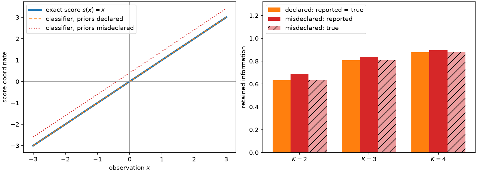
Left: the exact score map against two classifier-derived ones. The correctly declared classifier lies exactly on top of the exact score; the misdeclared one is offset by \(\log(1.5)/(2\delta)\). Right: for two, three and four cells, the retention a correctly declared classifier reports (which is also the truth) against the inflated number the misdeclared one reports and the information it actually retains.

This is why ScoreProvenance is not decoration. A classifier-derived provider always records kind="estimated_ratio", information_kind reads "supplied_score_surrogate", and no combination of arguments will make the library call an estimated quantity Fisher information. To measure what the labels truly retain, do what the snippet above does: label with the estimated score, then evaluate an exact score under those labels. Chapter 13 takes the estimated-ratio path seriously — how estimator quality maps to retention, what calibration diagnostics are worth running, and which parts of the question are genuinely open.

Choosing a door

Use Door 1 when the scores exist and you trust them; declare their provenance honestly. Use Door 2 whenever the model is differentiable, and prefer the integration source over a sample whenever the model is bounded and low-dimensional, since it removes Monte-Carlo noise from the answer entirely. Use Door 3 when there is no other way in — and then treat every number the library reports as conditional on the score estimate, because it is.

Runnable examples: door1-score-events, door2-mixture-densities, and door3-classifier walk each door end to end.

All three doors open onto the same room: a weighted table of score vectors. From here on the table is all that matters. Chapter 5 works out exactly how much information survives when that table is compressed into \(K\) labels.