Nuisance parameters: plain D against profiled \(D_s\)¶

This page is mostly about sample partitioning (optimize_partition), with space quantization (fit_quantizer) brought in at the end to supply a held-out column. It enters through Door 1, a precomputed table of (observation, score) events — although the scores here come from an exact component model, so Door 2 reaches the same table.

The measurement is a signal fraction. The obstacle is that the background shape is not known: two background components float alongside the signal, and nobody will ever quote them. That is the situation ProfiledDOptimality exists for, and this page measures what choosing it instead of plain DOptimality actually buys — in retained information, in a certified distance from the best possible answer, and in the width of the confidence interval a binned likelihood fit finally reports.

Two partitions, the efficient score, the certified ceiling, and the downstream fit

Problem¶

The reference density on \([0,1]\) is a mixture of one narrow signal peak and two truncated-exponential backgrounds with different rates,

\[\lambda(x;c) \;=\; c_{\text{sig}}\,\phi_{\text{sig}}(x) \;+\; c_{1}\,\phi_{1}(x) \;+\; c_{2}\,\phi_{2}(x),\]

with every \(\phi_k\) an exact normalized density and \(\sum_k c_k=1\), so \(c_{\text{sig}}\) is literally the signal fraction. The exact score at the reference coefficients is \(s_k(x)=\phi_k(x)/\lambda(x;c_0)\), which is what scores_from_components returns. Column 0 is the interest column; columns 1 and 2 are the nuisance columns, which is exactly the layout ProfiledDOptimality expects.

Two backgrounds rather than one is deliberate. With a single background the nuisance block is one-dimensional and the profiling correction is nearly a rescaling; with two similar exponential shapes the nuisance block is genuinely correlated with the interest direction, and profiling has something to do.

import numpy as np

import scorequant as sq
from examples.synthetic_problems import signal_background_shape

problem = signal_background_shape(
    background_rates=(1.0, 4.0), n_bins=4, sizes=(900, 300, 1500), seed=50
)
train, test = problem.train, problem.test
n_bins = problem.n_bins

assert problem.interest == (0,)
assert problem.nuisance == (1, 2)
assert train.scores.shape[1] == 3

Data and preprocessing¶

There is no preprocessing. The generator hands over observations, exact scores, and the reference intensity as each event's weight, and every fit below consumes those three arrays unchanged. Scores are never centered: the origin of score space carries the statement "this event is uninformative about this coefficient", which is a fact, not an offset.

Both criteria are scored by the same two public functions, on whatever labels they produce. information_report measures how much of the whole three-parameter Fisher matrix survives; profiled_information_report Schur-completes the two background columns out and measures how much information about the fraction survives. Neither function knows or cares which criterion made the labels, which is what makes the comparison fair.

One number is needed before any of them: the unbinned profiled information, which is the ceiling every retention below is measured against. It is a Schur complement of fisher_information and needs no partition at all.

from examples.nuisance_profiled_ds import score_labeling, unbinned_profiled_information

unbinned = unbinned_profiled_information(train.scores, train.weights, interest=problem.interest)
information = np.asarray(sq.fisher_information(train.scores, train.weights))

assert unbinned > 0.0
assert unbinned < information[0, 0]  # profiling can only remove information

API walkthrough¶

The same sample, two criteria¶

One call each. The only difference is the criterion object.

config = sq.DExchangeConfig(seed=11)

plain = sq.optimize_partition(
    train.scores,
    weights=train.weights,
    n_bins=n_bins,
    criterion=sq.DOptimality(),
    config=config,
)
profiled = sq.optimize_partition(
    train.scores,
    weights=train.weights,
    n_bins=n_bins,
    criterion=sq.ProfiledDOptimality(problem.interest),
    config=config,
)

plain_score = score_labeling(
    train.scores,
    np.asarray(plain.labels),
    train.weights,
    interest=problem.interest,
    n_bins=n_bins,
)
profiled_score = score_labeling(
    train.scores,
    np.asarray(profiled.labels),
    train.weights,
    interest=problem.interest,
    n_bins=n_bins,
)

assert plain_score.full_retention > profiled_score.full_retention
assert profiled_score.profiled_retention > plain_score.profiled_retention

Each criterion wins on its own objective and loses on the other one. That is the whole point, and it is worth stating in the negative: ProfiledDOptimality is not a better criterion. It answers a different question, and it pays for the answer with information about parameters you said you did not want.

The two partitions really are different objects, not two labelings of the same cells. Bin labels carry no meaning, so the comparison has to be through which rows are placed together, which the adjusted Rand index does.

from examples.nuisance_profiled_ds import interval_runs, partition_agreement

agreement = partition_agreement(np.asarray(plain.labels), np.asarray(profiled.labels), n_bins)
assert 0.2 < agreement < 0.95
assert interval_runs(train.observations, np.asarray(profiled.labels)) >= n_bins

The certified ceiling¶

Nothing above says how close either partition is to the best four-cell rule that exists. efficient_score_bound answers that, and it answers it with a certificate rather than an estimate. It builds the full-data efficient score \(\hat s = s_\psi - B^\ast s_\lambda\), partitions that one-dimensional coordinate exactly by weighted interval dynamic programming, and returns the resulting between-cell moment as a ceiling on the profiled objective of every four-cell rule of the whole three-dimensional score space.

bound = sq.efficient_score_bound(
    train.scores, interest=problem.interest, weights=train.weights, n_bins=n_bins
)
ceiling_retention = float(np.exp(bound.upper_bound - np.log(unbinned)))

assert bound.efficient_scores.shape == (train.scores.shape[0], 1)
assert bound.gap_to(profiled) >= -1e-9
assert profiled_score.profiled_retention <= ceiling_retention + 1e-9

The gap is reported in nats of the profiled log determinant, and gap_to refuses to compare against anything but a profiled partition on the same budget, because the two conventions would otherwise silently disagree.

The ceiling's labels as an initializer¶

The labels attaining the ceiling are not only a certificate. They already solve the relaxed upper problem, so handing them to optimize_partition starts profiled exchange inside the efficient-score geometry instead of at generic k-means seeding.

initialized = sq.optimize_partition(
    train.scores,
    weights=train.weights,
    n_bins=n_bins,
    criterion=sq.ProfiledDOptimality(problem.interest),
    config=config,
    initial_labels=bound.labels,
)

assert initialized.objective >= profiled.objective - 1e-12
assert bound.gap_to(initialized) <= bound.gap_to(profiled) + 1e-12
assert initialized.accepted_moves < profiled.accepted_moves

Supplied labels replace the seeding of the first restart only, so solver_restarts still explores; this is a head start, not a cage.

A held-out column needs two different solvers¶

Everything so far labels one fixed sample. PartitionResult has no predict_scores, on purpose. To say anything about events the solver never saw, you need a rule — and here the two criteria part company for a reason that is a theorem rather than a preference.

An exchange-stable D partition compiles: Chapter 8's Theorem 3 guarantees its labels are the training realization of a Mahalanobis nearest-cell rule, so compile_quantizer hands back that rule. A profiled partition has no such guarantee — Chapter 10 exhibits an eight-row table whose globally optimal profiled labeling puts a row in the wrong cell of the geometry it generates — so the library refuses to invent one.

try:
    initialized.compile_quantizer()
    raise AssertionError("a profiled partition has no canonical rule")
except ValueError as error:
    assert "no canonical inductive compilation" in str(error)

A reusable profiled rule therefore has to be fitted as one, which SoftVoronoiConfig does; that path is Chapter 12's subject and the soft-purification page's.

source = sq.ScoreSample(train.scores, train.weights)

d_rule = sq.fit_quantizer(
    source, n_bins=n_bins, criterion=sq.DOptimality(), config=sq.DExchangeConfig(seed=11)
)
ds_rule = sq.fit_quantizer(
    source,
    n_bins=n_bins,
    criterion=sq.ProfiledDOptimality(problem.interest),
    config=sq.SoftVoronoiConfig(seed=11, initializer_restarts=4, max_steps=120, record_every=60),
)

held_out = {
    name: score_labeling(
        test.scores,
        np.asarray(rule.predict_scores(test.scores)),
        test.weights,
        interest=problem.interest,
        n_bins=n_bins,
    )
    for name, rule in (("d", d_rule), ("ds", ds_rule))
}

assert held_out["d"].full_retention > held_out["ds"].full_retention
assert held_out["ds"].profiled_retention > held_out["d"].profiled_retention

The crossover survives out of sample, which is the only version of it that means anything.

Analysis¶

What each criterion retains¶

Full-study numbers, at four bins on 4000 training and 15000 held-out events, regenerated by examples/nuisance_profiled_ds.py into assets/nuisance-profiled-ds.json.

Labeling	Task	All three parameters	The fraction alone
Plain D	`optimize_partition`	0.94952	0.94855
Profiled \(D_s\), generic seeding	`optimize_partition`	0.90115	0.97903
Profiled \(D_s\), ceiling-initialized	`optimize_partition`	0.90115	0.97903
Plain D, compiled rule (held out)	`fit_quantizer`	0.95158	0.95005
Profiled \(D_s\), soft rule (held out)	`fit_quantizer`	0.93238	0.97358

Read the two columns against each other. Profiling gives up 4.84 points of overall D-efficiency and gets 3.05 points more information about the parameter that will be published. Whether that is a good trade is not a mathematical question; it is a question about what you are going to write down.

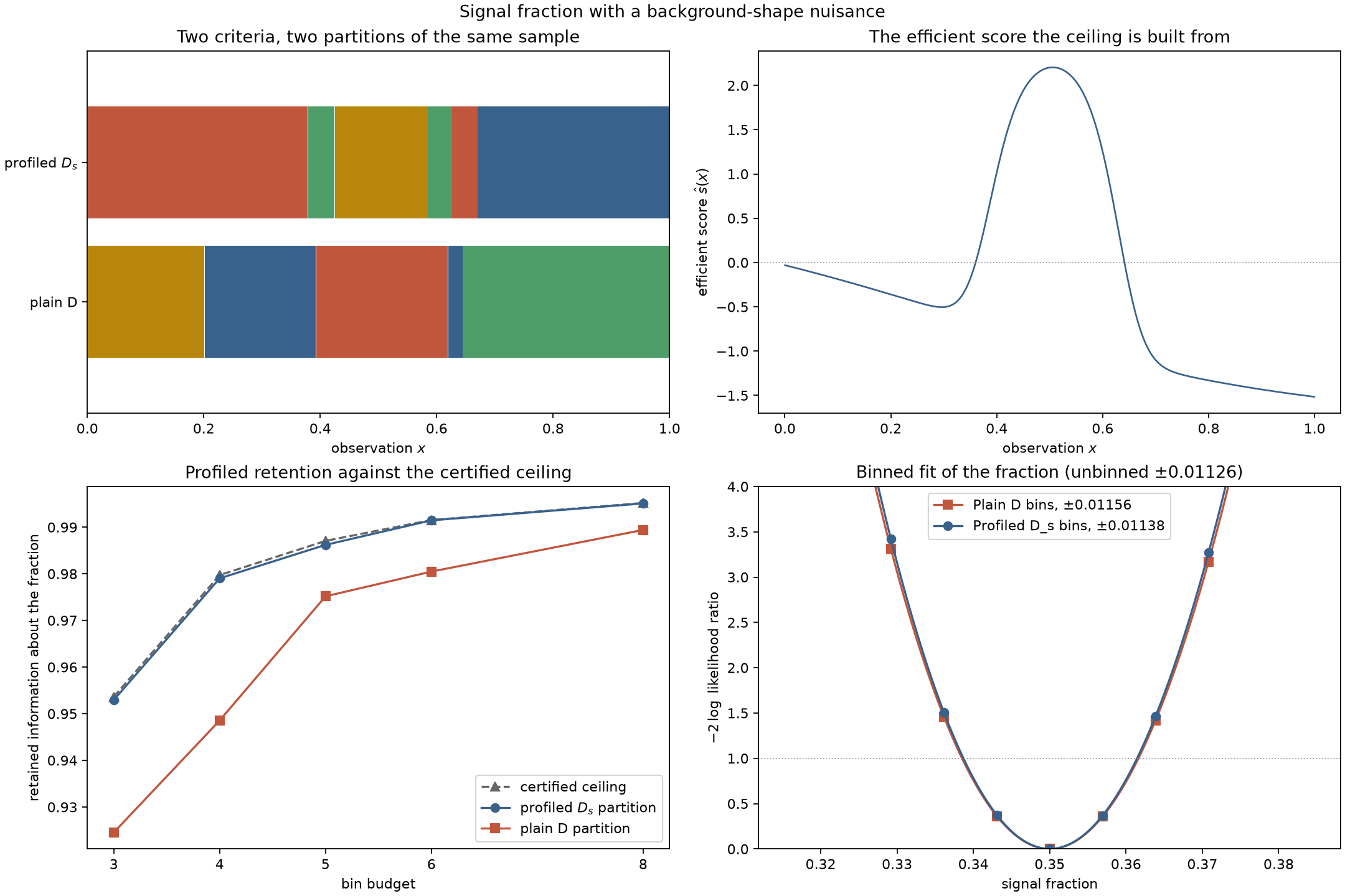
The two partitions place rows together very differently: their adjusted Rand index is 0.629, and where the plain-D partition needs five contiguous intervals of \(x\) to describe its four cells, the profiled one needs six.

The soft profiled rule is a restricted family — nearest-center cells — so it does not reach the free-label profiled partition's 0.97903; it reaches 0.97255 on training and 0.97358 on the held-out split. That is the honest price of insisting on a rule.

How close to the ceiling¶

The certified ceiling and the two profiled runs, over the bin budget:

Bins	Plain D	\(D_s\), generic seeding	\(D_s\), ceiling-initialized	Certified ceiling
3	0.92454	0.95294	0.95294	0.95364
4	0.94855	0.97903	0.97903	0.97972
5	0.97517	0.98504	0.98620	0.98706
6	0.98047	0.98591	0.99146	0.99153
8	0.98940	0.99322	0.99509	0.99518

Every column here is information about the fraction, so the ceiling applies to all of them. Three things fall out. Plain D is inefficient at this: it needs six bins just to match what profiled \(D_s\) already reaches with four (0.98047 against 0.97903). The ceiling is tight enough to be useful — the initialized profiled partition is within 0.0007 nat of a quantity no four-cell rule can exceed, which is 0.07% in ratio terms. And the certificate costs almost nothing: the exact scalar dynamic program on the efficient score is a one-dimensional problem.

What the initializer buys¶

Bins	Certified gap, generic seeding	Certified gap, initialized	Relocations, generic	Relocations, initialized
3	0.000735	0.000735	315	5
4	0.000710	0.000710	1715	17
5	0.002041	0.000867	672	23
6	0.005682	0.000071	631	24
8	0.001971	0.000096	870	51

Two different things happen, and they are worth keeping apart. At three and four bins the two runs converge on the same labeling, and the initializer only makes it cheaper — at four bins, 17 accepted relocations instead of 1715, and five scans instead of 26. At five, six, and eight bins the initializer also lands somewhere strictly better: at six bins it closes the certified gap by a factor of 80.

Neither effect is a guarantee, and the flat rows say so plainly. Profiled exchange is a local search; starting it inside the geometry of the relaxed problem it is trying to beat is a good heuristic, and the certificate is what turns "it converged" into "it is within 0.07% of unreachable".

What the measurement actually reports¶

None of the above is yet a confidence interval. So bin the data and fit.

The model is the one whose Fisher information the library has been optimizing all along: an extended Poisson likelihood over bin counts, \(\nu_b(c)=\sum_k c_k A_{bk}\), with \(A_{bk}\) the expected yield of component \(k\) in bin \(b\). The signal fraction is scanned; both background coefficients are profiled out at every scan point by the standard multiplicative expectation-maximization iteration for that model. The data are the expected counts at the reference coefficients, so this is an Asimov fit: it reports the interval the binning implies, not the outcome of one simulated experiment.

Because the model is exactly the one behind binned_fisher_information, the scan is checkable rather than merely illustrative — the half-width it finds must equal the reciprocal square root of the binned profiled information.

from examples.nuisance_profiled_ds import interval_study

study = interval_study(
    problem,
    {
        "d": ("Plain D", np.asarray(plain.labels)),
        "ds": ("Profiled D_s", np.asarray(initialized.labels)),
    },
    n_bins=n_bins,
)
rows = {row.key: row for row in study.rows}

for row in study.rows:
    assert abs(row.half_width - row.fisher_half_width) < 1e-4 * row.fisher_half_width
assert rows["ds"].half_width < rows["d"].half_width

At the full study size, with 4000 events in the sample:

Binning	68% interval half-width	Excess over the unbinned fit
Unbinned reference	0.011258	—
Four plain-D bins	0.011558	2.67%
Four profiled \(D_s\) bins	0.011376	1.04%

The profiled binning narrows the interval by 1.6%. Said the more informative way: binning at all costs 2.67% of precision on the fraction under plain D and 1.04% under profiled \(D_s\), so choosing the criterion that matches the measurement removes about three fifths of the price of binning — for free, at the same four bins, by changing one argument.

Do not inflate that. A 1.6% narrower interval is not a discovery; it is the size of effect this trade has at four bins on this problem. At eight bins the same two profiled retentions, 0.98940 and 0.99509, imply a narrowing of 0.29%, because by then there is very little left to win. The reason to care is that it costs nothing, and that the certificate tells you when there is nothing left to win.

Discussion¶

Task: sample partitioning is the main event (optimize_partition under both criteria); space quantization appears only to supply held-out numbers. Door: 1, precomputed score events. Criteria and solvers: DOptimality and ProfiledDOptimality with the exact positive-gain exchange, the exact scalar dynamic program inside efficient_score_bound, and SoftVoronoiConfig for the reusable profiled rule — every pairing one the dispatch table declares.

What the baselines did. The canonical baselines are not run here, and deliberately so: the solver shootout already establishes that any information-aware binning beats a rectangular observation grid by six to thirty D-efficiency points on this family of problems. The comparison this page needs is not naive-versus-informed but informed-versus-informed, and the meaningful reference point is not a baseline at all — it is the certified ceiling, which no rule of any kind can beat.

The honest caveat. There is no compile bridge for \(D_s\), and there will not be one. The finite profiled optimum is not forced into the geometry it induces: an exact rational eight-row fixture has a globally optimal profiled labeling that violates its own efficient-Voronoi rule by \(8/195\). The theory is Chapter 10, an optimum that violates its own geometry, and that fixture gets its own page in this section, ds-geometry-counterexample. Practically: a profiled partition is a fact about the rows you have, and a profiled rule is a different object that must be fitted as one.

The matching notebook, nuisance_profiled_ds.ipynb, runs the full-size study, prints every table above, and re-renders the figure.