Solver shootout: every method on one problem¶

This page runs both tasks — sample partitioning (optimize_partition) and space quantization (fit_quantizer) — through Door 1: a precomputed table of (observation, score) events. One two-parameter problem, every solver the library dispatches, and the three canonical baselines, scored the same way on the same held-out split.

It answers three questions a first-time user actually has. Does binning in score space beat binning the raw variables? Does the Fisher metric earn its keep, or would plain k-means do? And once you are inside the information-aware family, how much does the choice of solver matter?

Retention and cost of every solver and baseline

Problem¶

examples.synthetic_problems.two_parameter_gaussian_mixture places two overlapping isotropic Gaussian bumps on a bounded square. The reference measure is uniform over the square, each event's weight is the mixture intensity, and each event's score is the exact linear component score \(s_k(x)=\phi_k(x)/\lambda(x;c_0)\) from scores_from_components. Two components means two parameters and two score columns.

import numpy as np

import scorequant as sq
from examples.baselines import (
    equal_frequency_1d,
    euclidean_kmeans_scores,
    rectangular_observation_bins,
)
from examples.synthetic_problems import separable_1d_direction, two_parameter_gaussian_mixture

problem = two_parameter_gaussian_mixture(n_bins=16, sizes=(1_200, 600, 3_000))
train, test = problem.train, problem.test
n_bins = problem.n_bins
train.observations.shape, train.scores.shape

One structural fact governs everything below, so it is worth checking rather than asserting. An exact linear component score obeys \(\sum_k c_k s_k = 1\) identically: the reference coefficients contract the score vector to one. With two components that single identity pins the whole score cloud onto one affine line in the plane.

contracted = train.scores @ np.asarray([0.5, 0.5])
assert np.allclose(contracted, 1.0)
assert np.allclose(train.scores.sum(axis=1), 2.0)

The Fisher information is still full rank — scores are never centered, so the origin carries real information — but the variation in score space is one-dimensional. Keep that in mind when the whitening result arrives.

Data and preprocessing¶

Two methods work on a single score coordinate: the exact scalar dynamic program (ScalarDPConfig) and the equal-frequency baseline. Both get the same coordinate, the leading weighted-variance direction of the training scores, applied unchanged to the held-out split. This is a plain weighted principal direction, chosen because it is deterministic and stated openly — not because it carries any information guarantee.

direction = separable_1d_direction(train.scores, train.weights)
projected_train = (train.scores @ direction)[:, None]
projected_test = (test.scores @ direction)[:, None]
projected_train.shape, projected_test.shape

Every method below produces integer labels, and every label array is scored by the same public function, information_report, at the same bin budget. No baseline number is hand-rolled algebra.

def retention(scores: np.ndarray, labels: np.ndarray, weights: np.ndarray, bins: int) -> float:
    report = sq.information_report(scores, labels, weights, n_bins=bins)
    return float(report.geometric_mean_retention)

API walkthrough¶

Every applicable solver¶

The dispatch table in scorequant.api decides which configuration types each task accepts. optimize_partition accepts the two partition solvers; fit_quantizer accepts those two plus the three score-space solvers. Running the whole table is a loop over configurations, not five different call shapes.

source = sq.ScoreSample(train.scores, train.weights)
train_retention = {}
test_retention = {}

for name, config in [
    ("partition, exact D exchange", sq.DExchangeConfig(seed=7)),
    ("partition, guarded Mahalanobis-Lloyd", sq.MahalanobisLloydConfig(seed=7)),
]:
    partition = sq.optimize_partition(
        train.scores,
        weights=train.weights,
        n_bins=n_bins,
        criterion=sq.DOptimality(),
        config=config,
    )
    train_retention[name] = float(partition.report().geometric_mean_retention)

for name, criterion, config in [
    ("quantizer, exact D exchange", sq.DOptimality(), sq.DExchangeConfig(seed=7)),
    (
        "quantizer, guarded Mahalanobis-Lloyd",
        sq.DOptimality(),
        sq.MahalanobisLloydConfig(seed=7),
    ),
    (
        "quantizer, whitened k-means",
        sq.NormalizedTrace(),
        sq.KMeansConfig(seed=7, solver_restarts=8),
    ),
    (
        "quantizer, soft gradient descent",
        sq.DOptimality(),
        sq.SoftVoronoiConfig(seed=7, initializer_restarts=8, max_steps=120, record_every=30),
    ),
]:
    rule = sq.fit_quantizer(source, n_bins=n_bins, criterion=criterion, config=config)
    train_retention[name] = retention(
        train.scores, np.asarray(rule.predict_scores(train.scores)), train.weights, n_bins
    )
    test_retention[name] = retention(
        test.scores, np.asarray(rule.predict_scores(test.scores)), test.weights, n_bins
    )

PartitionResult has no predict_scores, on purpose: it labels one fixed sample and makes no claim about any other. That is why the two partition rows below carry a training number and no held-out number. The scalar dynamic program is the one solver that needs a different input — a single score column — so it takes the projection and is then scored against the full two-column score law, exactly like everything else.

scalar = sq.fit_quantizer(
    sq.ScoreSample(projected_train, train.weights),
    n_bins=n_bins,
    criterion=sq.DOptimality(),
    config=sq.ScalarDPConfig(seed=7),
)
train_retention["quantizer, scalar DP"] = retention(
    train.scores, np.asarray(scalar.predict_scores(projected_train)), train.weights, n_bins
)
test_retention["quantizer, scalar DP"] = retention(
    test.scores, np.asarray(scalar.predict_scores(projected_test)), test.weights, n_bins
)

spread = max(test_retention.values()) - min(test_retention.values())
assert min(test_retention.values()) > 0.99
assert spread < 2e-4

The three baselines¶

Each baseline is recomputed on each split from that split's own rows, which is deliberately generous: the baselines' "held-out" column is really an in-sample fit, and they still lose.

rectangular = rectangular_observation_bins(test.observations, total_budget=n_bins)
test_retention["baseline, rectangular observation bins"] = retention(
    test.scores, rectangular, test.weights, int(rectangular.max()) + 1
)
test_retention["baseline, Euclidean k-means on raw scores"] = retention(
    test.scores, euclidean_kmeans_scores(test.scores, n_bins, seed=7), test.weights, n_bins
)
test_retention["baseline, equal-frequency 1D bins"] = retention(
    test.scores, equal_frequency_1d(projected_test[:, 0], n_bins), test.weights, n_bins
)

best = max(value for name, value in test_retention.items() if not name.startswith("baseline"))
assert best - test_retention["baseline, rectangular observation bins"] > 0.03
assert best - test_retention["baseline, equal-frequency 1D bins"] > 5e-4

Analysis¶

Retention¶

Full-study numbers, at 16 bins on 4000 training and 15000 held-out events. The script examples/solver_shootout.py regenerates them into assets/solver_shootout.json.

Method	Task	Train D-efficiency	Held-out D-efficiency
Exact D exchange	`optimize_partition`	0.99916	not applicable
Guarded Mahalanobis-Lloyd	`optimize_partition`	0.99916	not applicable
Exact D exchange	`fit_quantizer`	0.99916	0.99910
Guarded Mahalanobis-Lloyd	`fit_quantizer`	0.99916	0.99910
Whitened k-means	`fit_quantizer`	0.99916	0.99910
Soft gradient descent	`fit_quantizer`	0.99916	0.99910
Scalar DP on the 1D projection	`fit_quantizer`	0.99917	0.99911
Rectangular observation bins	baseline	0.94226	0.93762
Euclidean k-means on raw scores	baseline	0.99906	0.99897
Equal-frequency 1D bins	baseline	0.99793	0.99788

A partition result has no held-out column because it deliberately has no predictor; the fit_quantizer row directly beneath it is the same solver compiled into a reusable rule, and reproduces the same training labels.

Cost¶

Timing methodology, stated so it can be argued with: one machine, one process, one warm-up call per method to absorb JAX tracing and compilation, then the median of five timed repetitions. Absolute seconds are hardware-specific and live in the JSON together with a machine note; only ratios belong in prose. Ratios are relative to the fastest information-aware fit.

Method	Relative cost per fit
Exact D exchange (`optimize_partition`)	1.00
Guarded Mahalanobis-Lloyd (`optimize_partition`)	1.01
Exact D exchange (`fit_quantizer`)	1.01
Guarded Mahalanobis-Lloyd (`fit_quantizer`)	1.01
Whitened k-means	1.03
Soft gradient descent	2.21
Scalar DP on the 1D projection	2.73
Rectangular observation bins	0.001
Euclidean k-means on raw scores	0.29
Equal-frequency 1D bins	0.001

This column is transcribed from the committed JSON and checked against it, so re-running the study on different hardware means regenerating both together. Treat the numbers as orders of magnitude, not as a benchmark.

The warm-up matters more than it sounds. Timed cold, the first exact-exchange fit takes several times its steady-state cost, because compilation dominates a problem this small. Reporting cold timings would have inverted the ranking. The measurement itself is one helper, and it is the same one the script uses:

from examples.solver_shootout import median_seconds

elapsed = median_seconds(
    lambda: sq.fit_quantizer(
        source, n_bins=n_bins, criterion=sq.DOptimality(), config=sq.DExchangeConfig(seed=7)
    ),
    3,
)
assert elapsed > 0.0

Claim 1: score space beats observation space¶

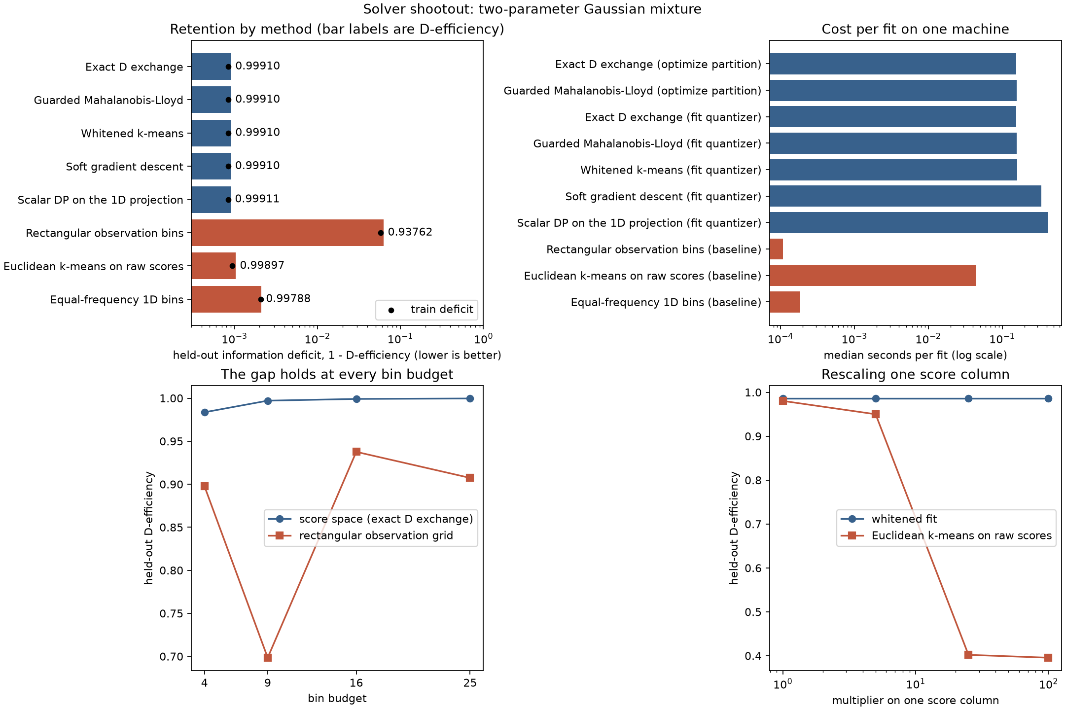
At 16 bins the best information-aware fit retains 0.99911 of the Fisher information; the equal-width 4-by-4 observation grid retains 0.93762. That is a gap of 6.1 D-efficiency points, and it understates the case: measured as information lost, the grid throws away about 70 times as much.

The gap is not an artifact of one bin budget. Across perfect-square budgets, where the grid always gets an exact cell count:

Bin budget	Score space (exact D exchange)	Rectangular grid	Gap
4	0.98360	0.89767	0.08594
9	0.99708	0.69843	0.29865
16	0.99910	0.93762	0.06148
25	0.99961	0.90734	0.09227

The grid is not merely worse; it is erratically worse. Its 9-bin value is far below its 4-bin value, because a 3-by-3 grid straddles the mixture's symmetry axis and produces cells whose score means nearly coincide. Adding cells to an observation-space grid does not reliably add information, which is the practical reason to stop tuning grids.

Claim 2: the metric matters, but you have to look where it can act¶

On this problem the raw-score Euclidean baseline loses only 0.00012 to the whitened k-means fit — a small gap that would be easy to over-read. It is worth saying plainly what that gap is not: it is not the whitening. Re-run the same weighted k-means with whitening turned off and the answer barely moves.

whitening = {}
for label, whiten in (("whitened", True), ("unwhitened", False)):
    rule = sq.fit_quantizer(
        source,
        n_bins=n_bins,
        criterion=sq.NormalizedTrace(),
        config=sq.KMeansConfig(seed=7, solver_restarts=8, whiten=whiten),
    )
    whitening[label] = retention(
        test.scores, np.asarray(rule.predict_scores(test.scores)), test.weights, n_bins
    )

assert abs(whitening["whitened"] - whitening["unwhitened"]) < 1e-3

In the full study those two differ by 0.0000082. The reason is the identity checked at the top of this page: with two components the score cloud lies on a line, every linear map acts along that line as a single uniform rescaling, and k-means partitions are invariant to a uniform rescaling. The metric has nowhere to act. What remains of the baseline's deficit is the reference measure it ignores — euclidean_kmeans_scores is unweighted, and these events carry very unequal weights.

To see whitening actually do something you need a score cloud with more than one direction of variation. Three components give one: the rescaling probe in the study runs signal_background_shape with two background shapes, multiplies the signal score column by a constant, and refits. Multiplying a score column is a reparameterization — a change of units for one coefficient — and D-efficiency is invariant under it, so any movement is a method reacting to units it should not be able to see.

Multiplier on one score column	Whitened fit	Euclidean k-means on raw scores
1	0.98581	0.98029
5	0.98581	0.94995
25	0.98581	0.40206
100	0.98581	0.39556

The whitened fit is invariant to twelve decimal places. The Euclidean baseline falls off a cliff: at a factor of 25 it retains 0.402, having lost 58 D-efficiency points to a change of units alone. Whitening is what buys that invariance, and the shootout's own problem simply has too little geometry to show it.

Claim 3: among information-aware solvers, the differences are small¶

All five information-aware fits land within 0.000011 of each other on the held-out split, and within 0.0000051 on training. On this problem the choice of solver is not a retention decision. It is a decision about cost and about guarantees:

Exact D exchange accepts only strictly improving single-row relocations, so it terminates exchange-stable and its D result compiles into a Mahalanobis rule.
Guarded Mahalanobis-Lloyd proposes whole relabelings and accepts one only when the exactly rebuilt objective improves. It matches exchange here at essentially the same cost.
Whitened k-means optimizes the normalized trace, not the determinant. It agrees here because the two criteria nearly coincide on this geometry; on a problem where they diverge it would not.
Soft gradient descent optimizes a relaxed objective and hardens at the end. It costs about twice as much and buys nothing measurable here.
The scalar dynamic program is the only globally exact solver in the table, but only on the one coordinate it is given. It reaches the best held-out number by a hair, which is what you would expect when the score law has a single direction of variation and the projection recovers it.

Small differences on one problem are not evidence that these solvers are interchangeable. They are evidence that this problem does not separate them. The counterexample pages show problems that do.

Discussion¶

Tasks: both. optimize_partition labels the fixed training sample; fit_quantizer returns a reusable rule with genuine held-out numbers. Door: 1, precomputed score events, though the scores come from an exact component model, so Door 2 would reach the same table. Criteria and solvers: DOptimality with exact exchange, guarded Mahalanobis-Lloyd, soft gradient descent, and the scalar dynamic program; NormalizedTrace with whitened k-means. Every pairing is the one the dispatch table declares.

What the baselines did. Rectangular observation bins lost 6.1 D-efficiency points and behaved non-monotonically in the bin budget. Euclidean k-means on raw scores was close here and catastrophic as soon as one score column changed units. Equal-frequency bins on the stated projection lost 0.0012 — the best of the three, and a reminder that a sensible one-dimensional summary is a real competitor when the score law is nearly one-dimensional.

What to take away. Choose score space over observation space; that is the decision worth 6 to 30 points here. Then choose a solver for its cost and its guarantees, and use a problem that actually separates solvers before believing a solver comparison. Chapter 14, Diagnostics and choosing a method, is the general version of this advice.

The matching notebook, solver_shootout.ipynb, runs the full-size study, prints both tables, and re-renders the figure.