5. Information after hard labels
From here the score is a vector. Chapter 4 closed with a weighted table of score rows, whatever door produced it, and the promise that the table is all that matters. This chapter cashes that promise: given the table and a rule that sorts its rows into \(K\) cells, exactly how much Fisher information do the resulting counts carry?
The answer is one formula. It is short enough to memorize, it is exact rather than asymptotic, and every criterion, algorithm, theorem, and diagnostic in the rest of the book is built on top of it. It is worth deriving carefully once.
The label has a likelihood of its own
Fix a hard rule \(q\) on score space and let \(Z=q(S)\) be the label of one event. The label is an ordinary random variable with an ordinary parametric law: it takes value \(b\) with probability
So the labeled experiment is a categorical model with \(K\) cells and the same parameter \(\theta\) as the original one. Its Fisher information is whatever the ordinary definition says it is; there is nothing to invent.
Differentiate the cell probability at the reference point, moving the derivative inside the integral (the rule does not depend on \(\theta\), so the indicator is a constant):
where the last equality names the cell score moment \(m_b=\mathbb{E}\big[S\,\mathbf{1}\{q(S)=b\}\big]\). Dividing by the cell probability gives the score of the discrete observation:
The conditional-score-mean identity. The score of a hard label is the average score of the events that produce it.
This is the tool the rest of the book leans on, so it is worth saying in words. Observing "the event landed in cell \(b\)" is evidence about \(\theta\) of exactly the strength that the typical member of cell \(b\) carries. Within-cell differences of opinion are averaged away and cannot be recovered. The identity is the geometric characterization of quantized Fisher information given by Barnes, Han and Özgür (2018), which the same authors then turned into information lower bounds for estimation under communication constraints (Barnes, Han and Özgür, 2020).
Summing the outer products of the label score over the label's own law gives the information the counts retain:
Three readings of the same object, each useful. The first says \(I_q\) is a weighted scatter of the \(K\) cell means about the score-space origin. The second says the whole problem depends on the rule through \(2K\) numbers only: \(K\) cell weights and \(K\) cell moment vectors. The third says information survives binning exactly to the extent that the cell means differ from the origin — which, when the score has mean zero as it does for a normalized model, is the same as the variance of the conditional mean. The third form is written uncentered anyway, because for an unnormalized intensity model the score's mean is not zero and subtracting it would delete the total-rate direction, as Chapter 4 showed.
The middle reading is the practical one. A rule with a million cells and a rule with four cells are compared through objects of the same size, and everything a criterion can see is the finite table \(\{(W_b, m_b)\}\). That is why the algorithms of Chapters 7 to 9 can be exact.
Checking the identity, not assuming it
For \(X\sim\mathcal N(\theta, I_2)\) at \(\theta_0=0\) the score is \(s(x)=x\), so score space is observation space and cell probabilities can be re-evaluated at a nearby \(\theta\) by tilting the same sample. Differencing \(\log W_b\) numerically must reproduce the conditional score mean.
import numpy as np

import scorequant as sq

rng = np.random.default_rng(15)
scores = rng.normal(size=(2_000, 2))  # X ~ N(theta, I) at theta0 = 0, so s(x) = x

partition = sq.optimize_partition(scores, n_bins=4, config=sq.DExchangeConfig(seed=0))
labels = np.asarray(partition.labels)
cell_weights = np.asarray(partition.cell_weights)
cell_means = np.asarray(partition.cell_score_means)


def log_cell_probability(theta, cell):
    """Log probability of one cell at theta, by exponential tilting of the sample."""
    tilt = np.exp(scores @ theta - 0.5 * theta @ theta)
    return np.log(np.mean(tilt * (labels == cell)))


delta = 0.02
for cell in range(4):
    gradient = []
    for coordinate in range(2):
        step = np.zeros(2)
        step[coordinate] = delta
        forward = log_cell_probability(step, cell)
        backward = log_cell_probability(-step, cell)
        gradient.append((forward - backward) / (2.0 * delta))
    assert np.max(np.abs(np.asarray(gradient) - cell_means[cell])) < 1e-3
The label's score really is the average score of its members, to the \(O(\delta^2)\) accuracy of a central difference. Now the matrix built from those means, against the library's own binned information:
by_hand = np.einsum("b,bp,bq->pq", cell_weights, cell_means, cell_means)
from_library = np.asarray(sq.binned_fisher_information(scores, labels, n_bins=4))

assert np.allclose(by_hand, from_library, rtol=0, atol=1e-9)
assert np.allclose(np.asarray(partition.information_partitioned), by_hand, rtol=0, atol=1e-9)
What the labels lose
Conditioning splits the second moment of the score, one term for each of the two things a label does and does not tell you:
Both terms are positive semidefinite, so \(I_q \preceq I_{\text{full}}\) always: hard labels can never manufacture information. The gap is the within-cell scatter, and it is the object every algorithm in this book is trying to make small.
Two conventions in that line are deliberate and both matter. The inner covariance is taken about the cell mean \(\mu_b\), because that is what the conditional expectation gives. The outer sum is not centered at all: \(I_{\text{full}}\) and \(I_q\) are uncentered second moments about the score-space origin. The origin of score space is where "this event says nothing about \(\theta\)" lives, and it is a statement about the model, not a convention. Subtracting a global mean from a score table would change the problem — Chapter 4 shows exactly how much — so ScoreQuant never does it, and neither does any formula in this book.
full = np.asarray(sq.fisher_information(scores))
scatter = sum(
    (scores[labels == cell] - cell_means[cell]).T @ (scores[labels == cell] - cell_means[cell])
    for cell in range(4)
)

assert np.max(np.abs(full - from_library - scatter)) < 1e-8
Refining a partition can never hurt
Split one cell in two. The pooled cell contributed \(m m^\top / W\) with \(m=m_1+m_2\) and \(W=W_1+W_2\); the two children contribute \(m_1m_1^\top/W_1 + m_2m_2^\top/W_2\). The matrix fractional map \((m,W)\mapsto mm^\top/W\) is jointly convex, and applying that convexity with weights \(W_1/W\) and \(W_2/W\) gives
with equality exactly when \(\mu_1=\mu_2\). Every other cell is untouched, so a refinement raises \(I_q\) in the Loewner order — the split gains nothing only when the two halves were saying the same thing anyway.
coarse_partition = sq.optimize_partition(scores, n_bins=3, config=sq.DExchangeConfig(seed=0))
coarse = np.asarray(coarse_partition.labels)
finer = coarse.copy()
finer[(coarse == 0) & (scores[:, 1] > 0.0)] = 3  # split cell 0 along the second coordinate

gain = np.asarray(sq.binned_fisher_information(scores, finer, n_bins=4)) - np.asarray(
    sq.binned_fisher_information(scores, coarse, n_bins=4)
)
assert np.min(np.linalg.eigvalsh(gain)) > -1e-9  # positive semidefinite up to rounding
This is the matrix version of the "refinement never hurts" fact Chapter 1 observed on a histogram. It is also the engine behind the global certificates of Chapter 8: treating every unassigned row as its own singleton cell produces a matrix that dominates every way of finishing the assignment, which is exactly what a branch-and-bound bound needs.
Rank: why \(K\) must exceed the number of parameters
For a normalized probability model the score has mean zero, so the cell moments sum to zero:
The \(K\) vectors \(m_1,\dots,m_K\) therefore span at most \(K-1\) dimensions, and since \(I_q\) is built from them,
A criterion that needs a nonsingular \(I_q\) — the log determinant of Chapter 8, above all — therefore needs at least \(d+1\) cells for \(d\) parameters. Two cells cannot measure two parameters, no matter where the boundary goes. Here is that wall, on a score table whose mean vanishes exactly by construction:
half = rng.integers(-9, 10, size=(600, 2)).astype(float)
symmetric = np.concatenate([half, -half], axis=0)  # E[S] = 0 holds exactly, in binary too
assert np.array_equal(symmetric.sum(axis=0), np.zeros(2))

two_cells = (symmetric[:, 0] > 0.0).astype(int)
two_cell_report = sq.information_report(symmetric, two_cells, n_bins=2)
assert two_cell_report.geometric_mean_retention == 0.0  # one direction is exactly dead
assert float(np.max(np.asarray(two_cell_report.retained_eigenvalues))) > 0.7  # the other is not

three_cells = sq.optimize_partition(symmetric, n_bins=3, config=sq.DExchangeConfig(seed=0))
four_cells = sq.optimize_partition(symmetric, n_bins=4, config=sq.DExchangeConfig(seed=0))
assert abs(float(three_cells.train_report.geometric_mean_retention) - 0.6006) < 0.01
assert abs(float(four_cells.train_report.geometric_mean_retention) - 0.7507) < 0.01
The collapse is structural, not numerical fragility to be tuned away: with two cells the two moment vectors are \(m\) and \(-m\), so \(I_q\) is exactly rank one and one whole direction of parameter space is invisible however the boundary is drawn. A third cell fixes it — recovering 60% of a two-parameter Fisher matrix from three counts, and 75% from four.
The D solver states the requirement rather than discovering it at run time. Asking for fewer cells than there are informative directions is refused by name:
three_parameters = rng.normal(size=(400, 3))
try:
    sq.optimize_partition(three_parameters, n_bins=2, config=sq.DExchangeConfig(seed=0))
    raise AssertionError("two cells cannot support three parameters")
except ValueError as error:
    assert "at least as many bins as informative directions" in str(error)
Reading the report
information_report assembles everything above for one labeling.
report = sq.information_report(scores, labels, n_bins=4)

assert report.effective_rank == 2
assert abs(float(report.geometric_mean_retention) - 0.6442) < 0.01
assert float(report.psd_residual_min_eigenvalue) > 0.0  # I_full - I_q is positive definite
assert np.array_equal(np.asarray(report.bin_counts), np.bincount(labels, minlength=4))
print(report)
The two retention numbers deserve to be told apart, because they are two different opinions about the same matrix. Both are computed after mapping into the informative subspace of \(I_{\text{full}}\) and whitening it, so the object being summarized is
whose eigenvalues lie in \([0,1]\) and are retained_eigenvalues. Then
arithmetic_mean_retention is their mean and geometric_mean_retention is their
geometric mean \(\exp(\tfrac1r\log\det R)\). The arithmetic mean is forgiving: a rule
that keeps one direction perfectly and loses another entirely still scores \(1/2\). The
geometric mean is not: it scores zero. Since a standard error is only as good as the
worst-measured direction of the parameter you claim to measure, the geometric mean is the
number this book quotes, and logdet_retention is its logarithm. Chapter
7 shows that the arithmetic mean is not merely a softer report but
a genuinely different design criterion with a different optimum.
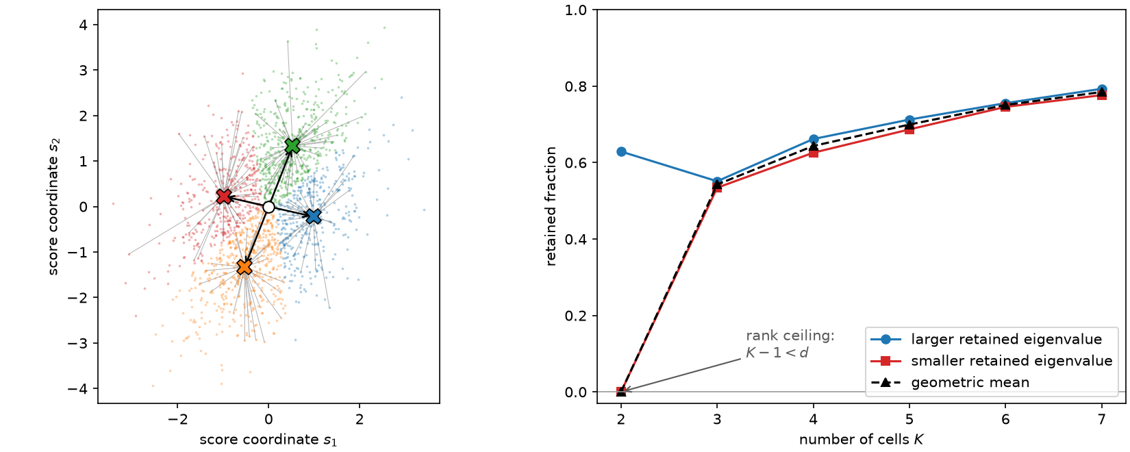
Left: a two-parameter score sample with four optimized cells. Information is the weighted scatter of the four cell means (crosses) about the score-space origin (circle); the grey segments are the within-cell residuals that the labels destroy. Right: the two retained eigenvalues and their geometric mean against the cell budget. Two cells leave one direction at exactly zero — the rank bound — and refinement lifts both.
The informative subspace, and why singular directions are projected out
Not every direction of a declared parameter space is measurable. A parameter can be exactly redundant (two components of a template that are proportional), or measurable only through a combination (a total rate and a fraction that enter the intensity the same way), or informative in principle but not in the reference sample. The Fisher matrix \(I_{\text{full}}\) then has an eigenvalue at or near zero, and \(I_{\text{full}}^{-1/2}\) does not exist.
ScoreQuant handles this by eigendecomposing \(I_{\text{full}}\) once, keeping the
directions whose eigenvalue exceeds rank_rtol times the largest, and working in that
subspace. Every result carries the resulting transform, so you can see what was kept:
redundant = np.concatenate([scores, scores[:, :1] * 2.0 - scores[:, 1:2] * 3.0], axis=1)
padded = sq.optimize_partition(redundant, n_bins=4, config=sq.DExchangeConfig(seed=0))

assert padded.transform.input_dim == 3
assert padded.transform.rank == 2
assert padded.transform.dropped_directions == 1
assert np.array_equal(np.asarray(padded.labels), labels)  # the third column changed nothing
assert (
    abs(
        float(padded.train_report.geometric_mean_retention)
        - float(partition.train_report.geometric_mean_retention)
    )
    < 1e-9
)
The third column was an exact linear combination of the first two. Projecting it out recovers the two-column answer exactly, labels included.
The alternative — adding \(\varepsilon I\) to \(I_{\text{full}}\) so that the inverse exists — is never used here, and the reason is not taste. A ridge invents information in a direction where the data has none. Retention is a ratio, and inflating its denominator by a fictitious \(\varepsilon\) makes every rule look better in a direction no rule can possibly measure; worse, the log determinant of a ridged matrix rewards a partition for spreading its cell means along the invented direction. Projection reports "this problem has rank two" and answers the rank-two question exactly. A ridge reports a rank-three number that is not about your experiment.
The threshold is a numerical decision and is exposed as one. rank_rtol defaults to
\(10^{-10}\) in double precision and \(10^{-5}\) in single, and the absolute cut actually
applied is transform.threshold. When a direction sits near that cut, the honest move is
to look at transform.eigenvalues and decide whether the parameterization is really
identified, not to nudge the tolerance until the answer changes.
What this buys
Everything from here is a choice of what to do with \(I_q\). A hard rule is a way of placing \(K\) cell means; the criterion is a scalar summary of the matrix they generate; the solver searches over rules. Chapter 6 settles a question that has to come first — whether you are labeling a table or building a rule, which are not the same task — and then Chapters 7 and 8 take the two summaries that matter, the trace and the log determinant, and show that they behave completely differently.