9. Mahalanobis geometry and guarded Lloyd

Chapter 8 ended with a theorem that practically begs to be turned into an algorithm. A terminal D partition is a Mahalanobis Voronoi diagram in the metric \(I_q^{-1}\). So: compute the metric, assign every row to its nearest cell mean in that metric, recompute the means and the metric, repeat. One full-data pass per iteration, no per-row scan, and a fixed point that satisfies the geometry the theorem describes.

This is the obvious algorithm, it is what Chapter 7's Lloyd iteration looks like when the metric is the one the criterion supplies, and it does not work. Not in the sense of being slow or fragile: one step of it can make \(\log\det I_q\) smaller. This chapter shows exactly how, explains why the usual proof fails, and describes the guard that makes the idea usable anyway.

The metric the criterion supplies

Before breaking it, it is worth understanding what \(I_q^{-1}\) is doing as a ruler.

The D metric weights each direction by the reciprocal of the information the current partition has already retained there. A direction that the cells are measuring well has a large eigenvalue in \(I_q\), hence a small one in \(I_q^{-1}\), so distances along it count for little; a direction the cells are measuring badly counts for a lot. Deciding which cell a row belongs to therefore emphasizes the parameter combinations the partition is currently worst at. That is the determinant criterion's whole personality in one sentence: it refuses to let any direction be neglected, because the product of the eigenvalues collapses if one of them does.

It also explains why the metric cannot be frozen honestly. Reassigning rows changes what is retained in each direction, which changes the ruler, which changes what "nearest" means. Chapter 7's Lloyd proof used a fixed metric in both of its two steps; here there is no fixed metric to use.

One batch step, downhill

Take the smallest configuration that shows it: eight rows, two parameters, three cells, equal weights. These numbers are a committed fixture rather than a lucky draw, and the whole demonstration is arithmetic.

import numpy as np

import scorequant as sq

scores = np.array(
    [
        [0.1116, 0.4427],
        [-0.2932, 0.6537],
        [-0.5995, -1.2685],
        [-0.6848, -1.5456],
        [0.4810, 0.9521],
        [1.6707, 0.9370],
        [0.1689, 1.7090],
        [-0.8548, -1.8805],
    ]
)
labels = np.array([1, 0, 0, 1, 2, 2, 2, 1])
weights = np.full(scores.shape[0], 1.0 / scores.shape[0])

information = np.asarray(sq.binned_fisher_information(scores, labels, weights, n_bins=3))
means = np.stack([scores[labels == cell].mean(axis=0) for cell in range(3)])
metric = np.linalg.inv(information)

Now do exactly what the theorem's geometry suggests: freeze that metric and send every row to its nearest cell mean in it.

residuals = scores[:, None, :] - means[None, :, :]
distances = np.einsum("nkp,pq,nkq->nk", residuals, metric, residuals)
batch = np.argmin(distances, axis=1)

before = float(np.linalg.slogdet(information)[1])
after = float(
    np.linalg.slogdet(np.asarray(sq.binned_fisher_information(scores, batch, weights, n_bins=3)))[1]
)

assert not np.array_equal(batch, labels)  # four rows change cell
assert abs(before - (-3.810643)) < 1e-6
assert abs(after - (-3.947164)) < 1e-6
assert after < before
print(round(before, 6), round(after, 6), round(after - before, 6))

The objective falls from \(-3.810643\) to \(-3.947164\): a loss of 0.136521 nat. The step did everything it was asked to do — each row really is now in its nearest cell under the metric it was given — and the criterion got worse.

What makes this more than a curiosity is that the step did improve the quantity it was actually optimizing. The frozen-metric distortion, the thing a nearest-centroid assignment minimizes, went down:

def frozen_distortion(assignment):
    """Weighted Mahalanobis within-cell distortion in the frozen metric."""
    offsets = scores - means[assignment]
    return float(np.einsum("np,pq,nq->", offsets, metric, offsets) / scores.shape[0])


assert frozen_distortion(batch) < frozen_distortion(labels)
print(round(frozen_distortion(labels), 4), round(frozen_distortion(batch), 4))

Distortion 13.55 before, 9.75 after — a 28% improvement in the surrogate, paid for with 0.14 nat of the objective. The surrogate and the objective are simply not the same function, and nothing forces them to move together.

Why the usual proof fails

The reason is one line of convexity, and it is worth writing out because it explains why no amount of care in implementing the batch step would fix it.

\(\log\det\) is concave on positive-definite matrices, so its first-order Taylor expansion is an upper bound:

\[\log\det I' \;\le\; \log\det I + \operatorname{tr}\!\big(I^{-1}(I'-I)\big) \qquad\text{for all } I' \succ 0 .\]

The nearest-centroid batch step is a step on that right-hand side. Improving an upper bound on a function tells you nothing whatsoever about the function: the bound can rise while the objective falls, and on this fixture it does exactly that.

batched = np.asarray(sq.binned_fisher_information(scores, batch, weights, n_bins=3))
tangent_change = float(np.trace(metric @ batched)) - scores.shape[1]

assert tangent_change > 0.0  # the surrogate went up
assert after - before < 0.0  # the objective went down
assert after - before <= tangent_change  # concavity, holding as it must
print(round(tangent_change, 4), round(after - before, 6))

The surrogate rose by 8.23 while the objective fell by 0.14, and the concavity inequality is satisfied throughout — nothing is broken, the bound is simply pointing the wrong way. A minorize-maximize argument needs the opposite: a lower bound that touches the objective at the current point, so that raising the bound must raise the objective. Concavity gives a majorizer, not a minorizer, and the direction of the inequality is not negotiable.

Contrast this with Chapter 7, where the metric was fixed and both Lloyd steps decreased the same function that the algorithm was minimizing. There was no surrogate, so there was nothing to diverge.

The guard

The repair is blunt and complete: never accept a batch proposal on the strength of the surrogate. Build the proposal, rebuild the exact criterion state from the proposed labels, and adopt it only if the exact objective strictly improved. That is MahalanobisLloydConfig, and the guard is part of the solver's contract rather than a safety option.

guarded = sq.optimize_partition(
    scores,
    weights=weights,
    n_bins=3,
    config=sq.MahalanobisLloydConfig(seed=0, guard="reject"),
    initial_labels=labels,
)

assert guarded.lloyd_iterations == 1  # the proposal was built
assert guarded.accepted_lloyd_steps == 0  # and rejected
assert np.array_equal(np.asarray(guarded.labels), labels)  # so nothing moved
assert guarded.exchange_stable is False

Started from the very labels that produce the counterexample, the guarded solver builds the same losing proposal, measures it exactly, and refuses it. The objective it reports is the one it started with — and honestly reports that the labels are not exchange-stable, which is why guard="reject" also refuses to compile them into a rule.

The default is guard="exchange", which hands the labels to the exact positive-gain engine of Chapter 8 once the batch stops improving. On this fixture the batch never improves at all, so the exchange does all the work — and there is plenty of it to do:

rescued = sq.optimize_partition(
    scores,
    weights=weights,
    n_bins=3,
    config=sq.MahalanobisLloydConfig(seed=0, guard="exchange"),
    initial_labels=labels,
)
history = np.asarray(rescued.objective_history)

assert rescued.accepted_lloyd_steps == 0
assert rescued.accepted_moves == 4
assert np.all(np.diff(history) > 0)
assert rescued.exchange_stable is True
assert rescued.objective > float(history[0]) + 2.7
print(round(float(history[0]), 6), round(rescued.objective, 6))

Four single-row relocations gain 2.78 nat, where the batch step would have lost 0.14. The starting configuration was simply a long way from stable, and single-row exchange found that out by evaluating exact gains instead of trusting a geometry that only holds at a terminal state.

One convention to keep straight when comparing these numbers with the ones above. The library optimizes in Fisher-whitened coordinates, so objective is \(\log\det\big(I_{\text{full}}^{-1/2} I_q I_{\text{full}}^{-1/2}\big)\), which differs from the raw \(\log\det I_q\) by the rule-independent constant \(\log\det I_{\text{full}} = -0.783062\) on this table. Differences — the \(-0.136521\) and the \(+2.78\) — are the same in either convention, which is why they are the numbers worth quoting.

full = np.asarray(sq.fisher_information(scores, weights))
offset = float(np.linalg.slogdet(full)[1])

assert abs(float(history[0]) + offset - before) < 1e-6
print(round(offset, 6))

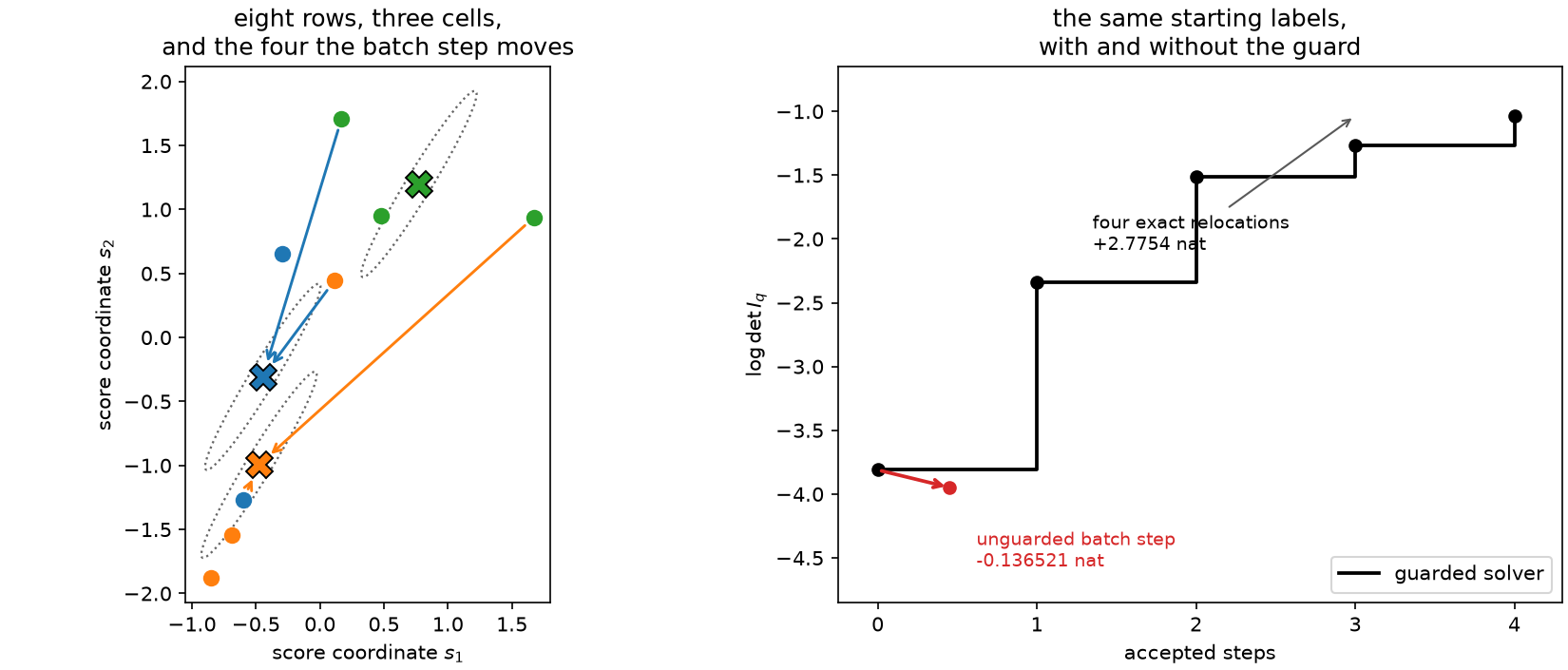
Left: the eight-row fixture with its three cells, their means (crosses), and one level set of the \(I_q^{-1}\) metric drawn at each mean — the same shape everywhere, because all cells share one metric. Arrows mark the four rows that a frozen-metric batch step relocates, coloured by destination; every one of them really is moving into a nearer cell. Right: the objective. The unguarded batch step loses 0.136521 nat in one move; the guarded solver rejects it and climbs 2.78 nat in four exact single-row relocations instead.

Empty cells, and what a guard has to catch

A frozen-metric proposal can also vacate a cell entirely, which the exact criterion state cannot represent at all — \(K\) cells with one of them empty is a \(K-1\)-cell partition with a singular \(I_q\) if \(K-1 < d+1\). The solver repairs such a proposal by keeping, for each emptied cell, the row it currently holds that is closest to its own centroid, so the recovered cell is the one the criterion currently supports best. A repair that empties some other cell as collateral is then rejected by the same guard as any other infeasible proposal.

This is worth naming because it is a second way the batch step can be wrong that has nothing to do with concavity, and both are caught by the same rule: propose freely, verify exactly, accept only improvements.

When to use which solver

With the guard in place both solvers are monotone and both terminate exchange-stable under the default guard="exchange", so the choice is about work per unit of progress rather than about correctness. They do different amounts of different things.

big = np.random.default_rng(41).normal(size=(20_000, 4))

lloyd = sq.optimize_partition(big, n_bins=6, config=sq.MahalanobisLloydConfig(seed=1))
exchange = sq.optimize_partition(big, n_bins=6, config=sq.DExchangeConfig(seed=1))

assert lloyd.exchange_stable and exchange.exchange_stable
assert abs(lloyd.objective - exchange.objective) < 0.01
print(
    lloyd.lloyd_iterations,
    lloyd.accepted_lloyd_steps,
    lloyd.scans,
    lloyd.accepted_moves,
    "|",
    exchange.scans,
    exchange.accepted_moves,
)

On this problem the guarded batch takes 51 full-data iterations, accepts almost all of them, and then needs only a handful of exchange scans to settle; the plain exchange takes 57 scans but relocates several thousand rows in the process, since its own batching moves many gain-ranked rows per scan. Both land on the same objective to within \(10^{-2}\).

The useful way to think about the difference:

• Guarded Mahalanobis-Lloyd makes large, coarse moves. Every iteration reconsiders every row at once, so it crosses a bad initialization quickly. It is the better choice when the starting labels are far from any sensible geometry, and when \(K\) is large enough that a per-row scan over all destinations is expensive.
• Exact exchange makes small, certified moves. Every accepted step is an exact improvement with a closed-form gain, so it does not need a rebuild to know whether a move helps, and it settles the boundary rows that a batch step keeps overshooting.

Neither escapes the basic limitation. Both are local, both depend on the seeding, and Chapter 8's certificates are the only thing in the library that answers the global question. Running both and keeping the better exact objective is cheap and is what the diagnostics workflow of Chapter 14 recommends.

The population picture, and what is missing from it

The batch iteration does have a clean theory — for a different objective. For squared-error quantization of a continuous law, the fixed points of Lloyd's algorithm are centroidal Voronoi tessellations: partitions in which each generator is the centroid of its own cell. Du, Faber and Gunzburger (1999) survey their structure and algorithms, and Du, Emelianenko and Ju (2006) prove convergence of the Lloyd iteration under explicit assumptions, continuing the line that starts with Lloyd (1982). That theory is what makes Chapter 7's fixed-metric iteration respectable.

None of it transfers here without work, and it is more honest to say so than to gesture at it. Those results are about an additive squared distortion with a fixed metric; the D objective is a nonlinear function of a matrix, with a metric that is a functional of the partition. For an absolutely continuous score law, moving a cell boundary does move positive probability mass, so shape derivatives can exist and the population first-order condition of Chapter 8 is meaningful — but a complete theorem giving differentiability with respect to moving generators, and convergence of a generator-space iteration to a local optimum, has not been established for the information criteria of this book. On a finite sample the situation is worse still, and for a reason that has nothing to do with concavity: the hard objective is piecewise constant in the generators, so it has no useful gradient anywhere. That is the observation Chapter 6 made when listing the three optimization levels, and it is what Chapter 12 does something about.

What survives from this chapter is a rule of practice with a proof behind it. Geometry that holds at an optimum is not a licence to iterate that geometry, because the metric moves with the partition. Propose with the geometry, verify with the criterion, accept only what improves. That discipline costs one exact rebuild per proposal and buys a monotone algorithm; the alternative costs 0.136521 nat on an eight-row table, and there is no reason to think it is bounded on a larger one.

Runnable example: lloyd-nonmonotone is the manuscript's counterexample, with the guard's acceptance trace rescuing monotonicity.

The next chapter changes the criterion rather than the solver. When only some of the parameters are of interest, profiling the rest away gives an objective that keeps the population geometry of Chapter 8 and loses its finite theorem — a different kind of gap, with a different repair.