Door 3: classifier-estimated density ratios, and what they honestly buy you

This page solves space quantization (fit_quantizer) through Door 3: density ratios estimated by a trained scikit-learn classifier, standing in for a likelihood ScoreQuant cannot evaluate. The classifier is one ratio backend among several — its calibrated posteriors over the training priors are the component density ratios, up to a factor that cancels. The page adds an actual retention-versus-classifier-quality ladder and an honest demonstration of the surrogate-information caveat from Chapter 13.

Problem

Events come from a two-component mixture, \(\lambda(x;\theta)=\theta_{\text{sig}}\phi_{\text{sig}}(x) +\theta_{\text{bkg}}\phi_{\text{bkg}}(x)\), with \(\phi_{\text{sig}}=\mathcal N(1.0, 0.5^2)\), \(\phi_{\text{bkg}}=\mathcal N(0.0, 1.5^2)\), and reference fractions \(\theta_0=(0.3,0.7)\). Unlike Door 2, the pdfs are treated as unavailable: only a classifier trained to separate labeled signal and background events stands in for them.

Data

Labeled training events are drawn per component to train the classifier; a separate, unlabeled sample is drawn from the reference mixture itself to fit and evaluate the quantizer. The classifier uses a quadratic feature \([x, x^2]\) so it can in principle reach the exact Bayes boundary between two different-variance Gaussians — the only thing the ladder below varies is how much labeled data it gets.

import numpy as np
from sklearn.linear_model import LogisticRegression

import scorequant as sq

signal_mu, signal_sigma = 1.0, 0.5
background_mu, background_sigma = 0.0, 1.5
reference_fractions = (0.3, 0.7)


def make_features(x):
    return np.column_stack([x, x**2])


def draw_reference_mixture(seed, n):
    rng = np.random.default_rng(seed)
    is_signal = rng.random(n) < reference_fractions[0]
    x = np.where(
        is_signal,
        rng.normal(signal_mu, signal_sigma, n),
        rng.normal(background_mu, background_sigma, n),
    )
    return x[:, None]


train_observations = draw_reference_mixture(2026, 400)
test_observations = draw_reference_mixture(999, 600)
train_observations.shape, test_observations.shape

API walkthrough

Train, wrap, and fit

Training and calibration stay application code; ScoreQuant starts at predict_proba, the declared training priors, and a declared parameterization. DensityRatioScore.from_classifier converts calibrated posteriors into density ratios and then into the mixture-fraction score.

def train_classifier(seed, n_per_class):
    rng = np.random.default_rng(seed)
    x_signal = rng.normal(signal_mu, signal_sigma, n_per_class)
    x_background = rng.normal(background_mu, background_sigma, n_per_class)
    x = np.concatenate([x_signal, x_background])
    y = np.concatenate([np.zeros(n_per_class), np.ones(n_per_class)])
    return LogisticRegression(max_iter=1000).fit(make_features(x), y)


def classifier_provider(model, description):
    def predict(x):
        return model.predict_proba(make_features(np.asarray(x)[:, 0]))

    return sq.DensityRatioScore.from_classifier(
        predict,
        [0.5, 0.5],
        sq.MixtureParameterization(list(reference_fractions)),
        description=description,
    )


small_model = train_classifier(101, n_per_class=15)
small_provider = classifier_provider(small_model, "logistic regression, 15 events per class")
small_result = sq.fit_quantizer(
    sq.ObservationSample(train_observations),
    provider=small_provider,
    n_bins=4,
    criterion=sq.DOptimality(),
    config=sq.DExchangeConfig(seed=7),
)
assert small_result.information_kind == "supplied_score_surrogate"

closure = sq.ratio_closure_report(
    small_provider.ratio(train_observations), np.ones(train_observations.shape[0])
)
assert round(closure.max_residual, 3) == 0.154  # visible estimator bias, before any fitting

information_kind is "supplied_score_surrogate" for every classifier-derived result, no matter how good the classifier is — kind="estimated_ratio" is recorded unconditionally, so the library never lets an estimate be reported as exact Fisher information. The ratio_closure_report line is the ratio-level diagnostic: exact ratios integrate to one under the training measure, so its residual bounds visible estimator bias from below before any quantizer is fitted.

The retention ladder

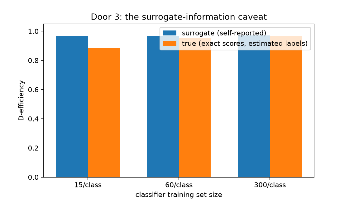
Refitting at three labeled training-set sizes shows the self-reported retention barely moving, while an independent check tells a different story.

def exact_posteriors(x):
    values = np.asarray(x)[:, 0]
    signal = np.exp(-0.5 * ((values - signal_mu) / signal_sigma) ** 2) / signal_sigma
    background = (
        np.exp(-0.5 * ((values - background_mu) / background_sigma) ** 2) / background_sigma
    )
    joint = np.stack([signal, background], axis=1)
    return joint / joint.sum(axis=1, keepdims=True)


exact_provider = sq.ScoreFunction(
    lambda x: sq.mixture_scores_from_ratios(
        sq.ratios_from_posteriors(exact_posteriors(x), [0.5, 0.5]), list(reference_fractions)
    ),
    provenance=sq.ScoreProvenance(kind="exact"),
)
oracle_test_scores = np.asarray(exact_provider.score(test_observations))

ladder = []
for n_per_class, seed in ((15, 101), (60, 102), (300, 103)):
    model = train_classifier(seed, n_per_class)
    provider = classifier_provider(model, f"logistic regression, {n_per_class} events per class")
    result = sq.fit_quantizer(
        sq.ObservationSample(train_observations),
        provider=provider,
        n_bins=4,
        criterion=sq.DOptimality(),
        config=sq.DExchangeConfig(seed=7),
    )
    surrogate = float(
        result.evaluate_scores(provider.score(test_observations)).geometric_mean_retention
    )
    labels = np.asarray(result.predict_scores(provider.score(test_observations)))
    true_retention = float(
        sq.information_report(
            oracle_test_scores, labels, n_bins=result.n_bins
        ).geometric_mean_retention
    )
    ladder.append((n_per_class, surrogate, true_retention))

small, medium, large = ladder
assert small[1] > 0.95 and small[2] < 0.90  # surrogate looks fine; the truth is not
assert large[2] > medium[2] > small[2]  # true retention rises with classifier quality
assert abs(large[1] - large[2]) < 0.01  # a good classifier's surrogate is finally trustworthy

# The table below rounds each ladder entry to three decimals.
assert [round(small[1], 3), round(small[2], 3)] == [0.966, 0.885]
assert [round(medium[1], 3), round(medium[2], 3)] == [0.969, 0.952]
assert [round(large[1], 3), round(large[2], 3)] == [0.970, 0.966]

# The ceiling a quantizer fit directly from the exact score reaches on this sample.
direct = sq.fit_quantizer(
    sq.ObservationSample(train_observations),
    provider=exact_provider,
    n_bins=4,
    criterion=sq.DOptimality(),
    config=sq.DExchangeConfig(seed=7),
)
direct_retention = float(
    direct.evaluate_scores(exact_provider.score(test_observations)).geometric_mean_retention
)
assert round(direct_retention, 3) == 0.972

Analysis

Training size	Surrogate retention	True retention (exact scores, estimated labels)
15 / class	~0.966	~0.885
60 / class	~0.969	~0.952
300 / class	~0.970	~0.966

The surrogate number — what evaluate_scores reports on the classifier's own estimated scores — stays close to 0.97 throughout, because it measures \(\operatorname{Var}(E[\hat s\mid q(\hat s)])\): how well the bins preserve the estimated score, which the D-optimal solver is genuinely good at regardless of how good the estimate is. The true number relabels the same held-out events with the classifier-based bins, then scores the exact mixture-fraction score under those labels — \(\operatorname{Var}(E[s\mid q(\hat s)])\) — and it is what a real downstream fit's information actually depends on. At 15 labeled events per class the gap is 8 points of D-efficiency; by 300 it has closed to under one point, converging on the same ceiling a quantizer fit directly from the exact score reaches (~0.972 on this sample).

Discussion

Task: space quantization (fit_quantizer). Door: 3, classifier-derived density ratios via DensityRatioScore.from_classifier with a MixtureParameterization. Criterion / solver: DOptimality with exact exchange, held fixed across the ladder so only classifier quality varies.

The caveat is not a defect to work around; it is what information_kind == "supplied_score_surrogate" is warning about on every classifier-backed result. Trust the self-reported retention only as far as you trust the classifier — and when you can, check it the way this page does: relabel a held-out sample with the fitted rule, then evaluate an exact or better-estimated score under those labels. See Chapter 13 for which parts of classifier error cost information and which do not.

The matching notebook, door3_classifier.ipynb, runs a longer ladder at full sample size and plots the convergence directly.