A profiled optimum outside its own geometry

This page is about sample partitioning only (optimize_partition), and it enters through Door 1: a score table, eight rows of it, written down rather than sampled. It exists to make one exact result runnable, and the result is the reason the library has no compile bridge for the profiled criterion. The theory is Chapter 10.

For the plain determinant, Chapter 8's Theorem 3 says that exchange stability forces geometry: a stable labeling cannot contain a misplaced row, so its labels are the training realization of a Mahalanobis nearest-cell rule and compile_quantizer can hand that rule back. The natural conjecture is that the same holds for profiled \(D_s\) with its efficient semimetric in place of the Mahalanobis one.

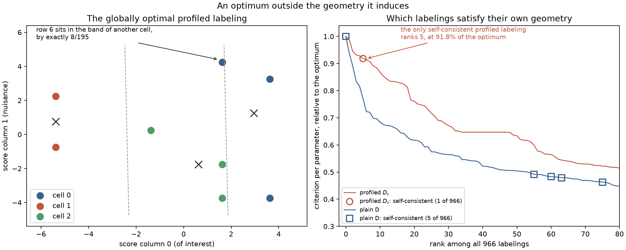
It does not. On the eight rows below, the labeling that maximizes the profiled objective over all 966 three-cell labelings puts one row strictly in another cell's region of the geometry that this very labeling induces, by an exact rational \(8/195\). Every quantity on this page is computed with fractions.Fraction, so no sign depends on a tolerance.

Problem

The parameter of interest is score column 0; column 1 is a nuisance to be estimated from the same labels and profiled away. The criterion is the scalar Schur complement

\[S(I_q)\;=\;(I_q)_{00}-\frac{(I_q)_{01}(I_q)_{10}}{(I_q)_{11}},\]

whose logarithm is what ProfiledDOptimality((0,)) maximizes. The question is whether the best labeling of a finite table has to satisfy the nearest-cell rule in the semimetric it generates. The way to settle that on eight rows is to enumerate every labeling.

Data and preprocessing

There is none, and there is nothing to normalize. The fixture is constructed: eight integer vectors, shifted once by their own exact mean so that the table sums to zero the way a score sample from a normalized model does under its own reference measure. That shift is part of the construction of a plausible score table, not preprocessing applied to data — scores are never centered by this library, because the score-space origin means "this event says nothing about these parameters".

Working in integers keeps every derived quantity a rational with a small denominator, which is what makes the whole demonstration exact.

from fractions import Fraction

from examples.ds_geometry_counterexample import (
    RAW_TABLE,
    canonical_labelings,
    exact_table,
    profiled_value,
)

table = exact_table()
labelings = canonical_labelings()

assert len(RAW_TABLE) == 8
assert all(len(row) == 2 for row in table)
assert [sum(row[column] for row in table) for column in (0, 1)] == [Fraction(0), Fraction(0)]
assert len(labelings) == 966

Bin names carry no meaning, so labelings are enumerated in restricted-growth form: row 0 is in cell 0, and a new cell may only be opened by the smallest unused index. That visits every three-cell partition of eight rows exactly once instead of once per relabeling, which is why 966 is the count of partitions rather than of label vectors.

API walkthrough

The exact global optimum

Rank all 966 by the exact profiled value. The winner is clear-cut: it beats the runner-up by \(2929/21120\), which is about 0.139 in absolute terms and leaves no room for a numerical accident.

ranked = sorted(((profiled_value(labels, table), labels) for labels in labelings), reverse=True)
best, optimum = ranked[0]

assert optimum == (0, 1, 2, 1, 2, 0, 0, 2)
assert best == Fraction(20449, 1920)
assert best - ranked[1][0] == Fraction(2929, 21120)
assert round(float(Fraction(2929, 21120)), 3) == 0.139

The geometry that optimum induces

The gradient of the profiled objective at a labeling is the inverse binned information minus the embedded inverse of its nuisance block. Here it has rank one, so its level sets are parallel bands of constant efficient score — the interest column with the nuisance column regressed out. Ask where each row belongs under the bands that the optimum itself generates.

from examples.ds_geometry_counterexample import efficient_semimetric, violation_margins

semimetric = efficient_semimetric(optimum, table)
margins = violation_margins(optimum, table, semimetric)

assert semimetric is not None
assert margins[6] == Fraction(8, 195)
assert sum(margin > 0 for margin in margins) == 1
assert all(margin == 0 for margin in margins[:6] + margins[7:])

Row 6 is labeled 0, and in the semimetric that cell 0 helped create it is strictly closer to cell 2 — by an exact positive rational. Moving it there would satisfy the geometry and would lower the objective, because the labeling it is leaving is the global optimum. There is no tolerance to blame and no local-search artifact to appeal to.

The library reproduces it, and measures the violation

The same eight rows in floating point, solved from a cold start, land on the same partition and report the violation as a measured quantity rather than a promise.

import numpy as np

import scorequant as sq
from examples.ds_geometry_counterexample import float_table

scores, weights = float_table()
profiled = sq.optimize_partition(
    scores,
    weights=weights,
    n_bins=3,
    criterion=sq.ProfiledDOptimality((0,)),
    config=sq.DExchangeConfig(seed=1, initializer_restarts=32, max_scans=200),
)
geometry = profiled.profiled_geometry

assert np.array_equal(np.asarray(profiled.labels), np.asarray(optimum))
assert abs(float(np.exp(profiled.objective)) - float(best)) < 1e-10
assert geometry.violating_moves == 1
assert abs(geometry.maximum_positive_violation - float(Fraction(8, 195))) < 1e-12

The same report carries the quantitative side of the story. Chapter 10's proposition bounds the violation at a stable labeling by the row's own leverage, roughly the number of cells divided by the number of rows; maximum_bound_residual is the largest violation minus its own bound, and the proposition makes it nonpositive.

assert geometry.maximum_bound_residual <= 0.0
assert geometry.bound_certified is True

With an eighth of the total mass on every row, the bound here is loose enough to permit a violation of this size. That is exactly why the counterexample lives on eight rows.

The refusal

compile_quantizer exists because Theorem 3 makes it bookkeeping. Without a theorem there is nothing to compile, and the library says so instead of returning a nearest-cell rule that would disagree with the labels it came from.

try:
    profiled.compile_quantizer()
    raise AssertionError("a profiled partition has no canonical rule")
except ValueError as error:
    assert str(error) == (
        "finite profiled-D labels have no canonical inductive compilation; "
        "fit an explicit quantizer instead"
    )

The same eight rows under plain D

Change one argument and the missing implication comes back. The determinant partition of the same table is self-consistent, compiles, and — this being an eight-row problem — can be proved globally optimal outright.

plain = sq.optimize_partition(
    scores,
    weights=weights,
    n_bins=3,
    config=sq.DExchangeConfig(seed=1, initializer_restarts=32, max_scans=200),
)
certificate = sq.certify_partition(scores, weights=weights, n_bins=3, incumbent=plain.labels)
compiled = plain.compile_quantizer()

assert plain.geometry.voronoi_consistent is True
assert plain.geometry.violating_moves == 0
assert np.array_equal(np.asarray(compiled.predict_scores(scores)), np.asarray(plain.labels))
assert certificate.status == "optimal"
assert certificate.incumbent_was_optimal is True

The exact enumeration agrees, and says the same thing without any solver in the way.

from examples.ds_geometry_counterexample import determinant_value, mahalanobis_metric

d_ranked = sorted(
    ((determinant_value(labels, table), labels) for labels in labelings), reverse=True
)
d_best, d_optimum = d_ranked[0]
d_margins = violation_margins(d_optimum, table, mahalanobis_metric(d_optimum, table))

assert d_best == Fraction(71289, 1024)
assert all(margin == 0 for margin in d_margins)

Analysis

How rare is a self-consistent labeling?

The enumeration answers a sharper question than "does the optimum violate its geometry". It can ask how many of the 966 labelings satisfy their own, under each criterion. Two of the 966 have a singular binned information and induce no geometry at all; of the remaining 964:

from examples.ds_geometry_counterexample import rank_labelings

profiled_survey = rank_labelings("profiled", table)
determinant_survey = rank_labelings("determinant", table)

assert profiled_survey.singular_labelings == 2
assert len(labelings) - profiled_survey.singular_labelings == 964
assert profiled_survey.consistent_ranks == [5]
assert determinant_survey.consistent_ranks == [0, 55, 60, 63, 75]
assert determinant_survey.optimum_is_consistent is True
assert profiled_survey.optimum_is_consistent is False

Criterion	Self-consistent labelings	Rank of the best one	Its value, relative to the optimum
Plain D	5 of 966	0	1.000000
Profiled \(D_s\)	1 of 966	5	0.918327

Read the profiled row carefully, because it is stronger than the headline. On this table the efficient-Voronoi geometry does not merely fail to contain the optimum: exactly one labeling of 966 satisfies it, and that labeling is fifth-best, retaining 91.83% of the profiled information the optimum retains. In log terms it is 0.0852 nat short. A solver constrained to produce geometrically self-consistent profiled labelings would, on this table, have exactly one choice, and it would be the wrong one.

import math

assert abs(profiled_survey.best_consistent_ratio - 0.918327) < 1e-6
assert abs(-math.log(profiled_survey.best_consistent_ratio) - 0.085201) < 1e-6

The plain-D row is Theorem 3 in the form the theorem actually takes. Self-consistency is necessary at an optimum but not sufficient: five labelings satisfy the Mahalanobis rule, four of which are merely locally reasonable and rank 55th or worse. The theorem says the optimum is among them, and it is — at rank 0.

Where Chapter 8's proof dies

The D proof turns on a coincidence between the determinant lemma's coefficients and the leverage bound. Subtracting the nuisance block's log determinant subtracts a second determinant-lemma gain, computed with its own coefficients in the nuisance block, and the two sides no longer meet. Concretely, a relocation can hurt the full determinant a little and help the nuisance determinant more; the efficient semimetric, which sees only the difference through the gradient, cannot see that happening.

Nothing else breaks. The exchange gain for \(D_s\) is still exact and still closed-form, the solver is still monotone, and it still terminates — those are statements about the algebra of a rank-two update, and they do not depend on any geometry. What is missing is only the bridge from a stable labeling to a rule.

Discussion

Task: sample partitioning, and nothing else. That is the point rather than a limitation: a profiled partition is a fact about the rows you have, and this page is about why it cannot quietly become more than that.

Door: 1. The table is a bare score matrix, constructed rather than generated.

Criterion and solver: ProfiledDOptimality((0,)) with DExchangeConfig, plus DOptimality and certify_partition for the contrast. Everything else is exact rational arithmetic that no solver touches.

What the baselines did. They are not run. The reference point here is not a naive binning but an exhaustive enumeration, which is stronger than any baseline: it is the whole feasible set.

What to do instead. A reusable profiled rule has to be fitted as one, which SoftVoronoiConfig does — an honest inductive fit with a validation report rather than a finite labeling wearing a rule's clothes. That path is Chapter 12's subject and is measured on a real measurement problem in nuisance-profiled-ds, where the fitted rule's shortfall against the free-label partition is exactly the price of insisting on a rule.

The matching notebook, ds_geometry_counterexample.ipynb, runs both enumerations, prints the tables above, and re-renders the figure.