Problem and data

FlowCyt contains 30 bone-marrow samples and five expert-annotated target populations. We retain the remaining cells as a sixth other component. This matters: removing other using the expert labels would leak the answer before inference starts.

Licence and provenance

The FlowCyt paper describes the benchmark and its expert populations. The data, and therefore every sample derived from them in this study — the committed CI fixture included — are licensed under CC BY-NC-SA 4.0, separately from ScoreQuant's MIT-licensed code. Copyright belongs to Lorenzo Bini, Fatemeh Nassajian Mojarrad, Margarita Liarou, Thomas Matthes, and Stéphane Marchand-Maillet. The upstream corpus lives in the FlowCyt classification benchmark repository.

Every generated manifest records the source URLs, file totals, sampling settings, and digest, so a derived sample can always be traced back to the licensed original. Redistribution of the derived samples carries the same non-commercial share-alike terms as the source.

The bounded 600,000-cell sample

The public corpus stores every patient/population pair in a separate FCS file. Downloading and unpacking the complete archive is unnecessary for this bounded study. The acquisition command reads FCS metadata first, allocates exactly 20,000 cells per patient in proportion to the upstream component totals, and then range-reads 16 deterministic strata within every nonempty component. Largest-remainder allocation keeps every sampled population fraction within \(3.4\times10^{-5}\) of its full-file fraction.

uv run python -m examples.cell_population \
  --download-sample flowcyt-results/flowcyt_sample_20000.npz \
  --max-per-patient 20000 \
  --sample-blocks 16 \
  --download-workers 12

This is component-stratified acquisition, not label-blind acquisition. The expert component totals determine how many rows are read so that rare classes are not lost to coarse network sampling. Once the 600,000-row dataset is assembled, test labels are absent from classifier fitting, score calibration, partition learning, template estimation, and mixture inference. They return only for the final comparison with expert fractions.

The bounded sample SHA-256 is a08e9bf183fe32b913e155d413eeacfdb65c7f99017a42e69c4b91bdde20d987. The file itself is deliberately not committed; the digest and the command above are what make it reproducible.

The frozen patient split

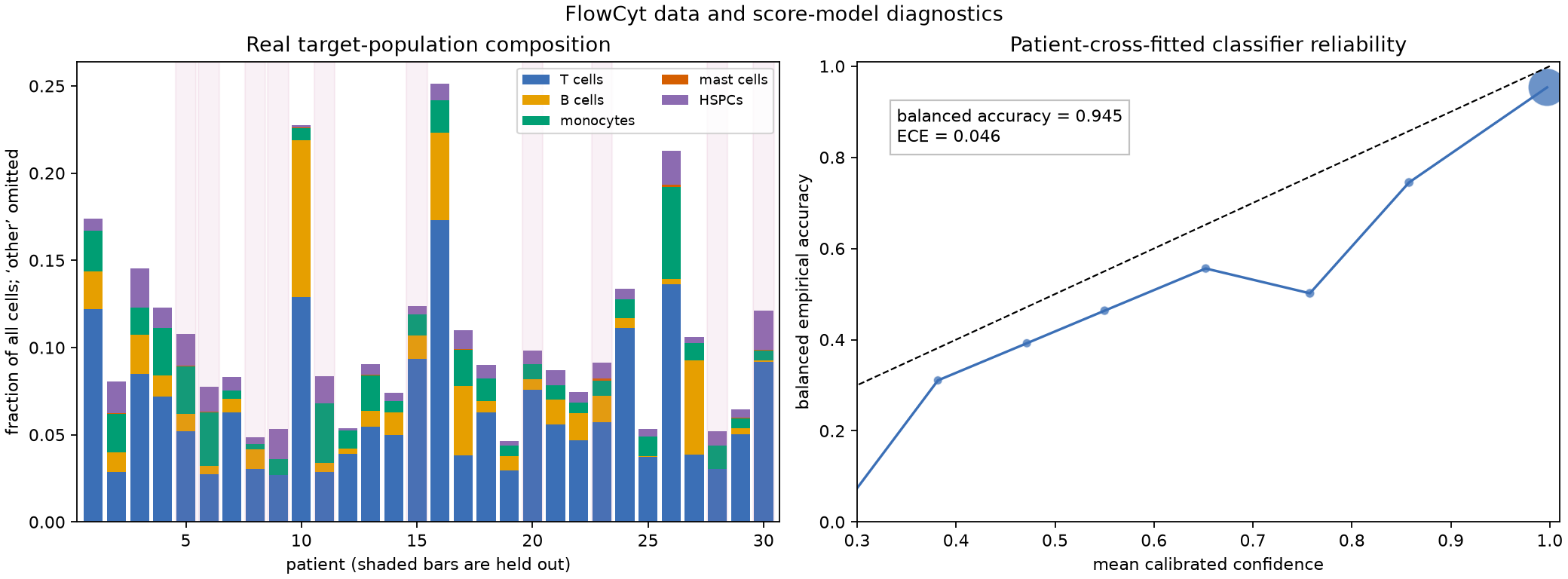
The shaded bars are the ten test patients. The target composition varies substantially: T cells range from roughly 2.7% to 17.3% across the cohort, while mast cells are often below 0.02%. This is one reason an ordinary random row split would be misleading. The split must happen by patient.

The exact frozen patient split is:

• reference: 1, 2, 3, 4, 7, 10, 12, 13, 14, 16, 17, 18, 19, 21, 22, 24, 25, 26, 27, 29;
• test: 5, 6, 8, 9, 11, 15, 20, 23, 28, 30.

Within the reference cohort, five four-patient folds produce out-of-fold score predictions. Calibration selection is nested: each outer patient fold is absent from classifier fitting and from the inner out-of-fold calibration used to score it. Disjoint deterministic row roles are then used for partition fitting, validation diagnostics, and bin-template estimation. Validation rows never affect gradients, stopping, or checkpoint selection.

The reference composition \(\theta_0\) that the integration measure reproduces is dominated by other, which is what makes the five target directions worth learning at all:

Population	Reference fraction
T cells	0.0711
B cells	0.0196
Monocytes	0.0150
Mast cells	0.00019
HSPCs	0.00812
Other	0.8860

The committed CI fixture

Continuous integration never touches the 600,000-cell sample. It uses a small committed fixture, examples/data/flowcyt_fixture.npz, with 34,554 cells drawn from the same 30 patients under the same frozen split. Its licence and provenance notes live beside it in examples/data/README.md, and its sampling details are recorded in examples/data/flowcyt_fixture.json.

JAX_ENABLE_X64=1 MPLBACKEND=Agg \
  uv run python -m examples.cell_population \
  --fixture examples/data/flowcyt_fixture.npz \
  --quick

The fixture is class-balanced rather than composition-faithful, so its reference composition is near-uniform across the five target populations. Fixture-scale numbers therefore demonstrate that the code path runs and that the qualitative conclusions hold; they are not the study's quantitative result. Every published number in this section states which of the two scales it came from.

The full-corpus transport audit

The full CSV corpus can be reconstructed directly from the public component FCS files. The downloader streams each component instead of materializing a patient in memory, writes atomically, and records every row count and SHA-256:

uv run python -m examples.cell_population \
  --download-full-csv-dir flowcyt-results/data_original \
  --download-chunk-rows 200000 \
  --download-workers 6

This produced all 30 Case_*.csv files: 21,254,866 events and about 3.9 GB of CSV data. The files remain ignored local evidence. The separate chunked audit then reads every row, compares per-patient class fractions and marker moments with the frozen 600k sample, and makes no fit, calibration, or tuning decision:

uv run python -m examples.cell_population \
  --data-dir flowcyt-results/data_original \
  --transport-audit-sample flowcyt-results/flowcyt_sample_20000.npz \
  --transport-audit-output flowcyt-results/full_transport_audit.json \
  --transport-audit-chunksize 200000

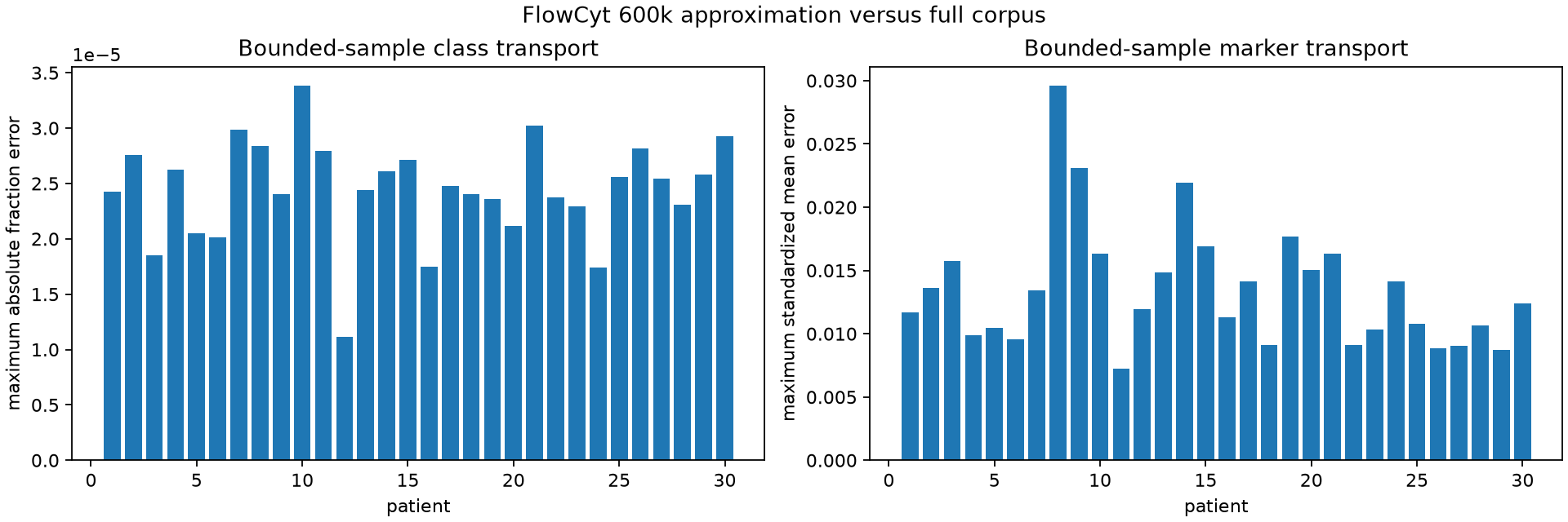
The completed audit found a maximum absolute patient/class fraction error of \(3.39\times10^{-5}\) and a maximum absolute standardized marker-mean error of 0.0296. Thus the deterministic component-stratified sample is exceptionally accurate for class composition and within 0.03 pooled standard deviations for every audited patient/marker mean. This validates the bounded measure as a transport approximation for the reported low-order moments; it does not prove that every nonlinear score-space boundary or rare tail is transported equally well.

import json
from pathlib import Path

transport = json.loads(Path("docs/usecases/assets/flowcyt_transport_audit.json").read_text())

assert transport["full_corpus"]["rows"] == 21_254_866
assert len(transport["full_corpus"]["files"]) == 30
assert round(transport["maximum_absolute_class_fraction_error"], 7) == 3.39e-05
assert round(transport["maximum_absolute_standardized_feature_mean_error"], 4) == 0.0296
assert "no tuning" in transport["purpose"]

The committed JSON evidence contains the SHA-256 and row count of every full-corpus CSV, the bounded-sample digest, and all patient-level diagnostics. The compact CSV table supports independent plotting. These are stress-audit results, not another opportunity to choose the frozen patient split, classifier, calibration, bin count, or quantizer.

The connection to the theory is precise. The information identity in Chapter 5 depends on cell masses and score first moments, while the empirical-consistency statement in Chapter 12 requires control of the underlying score law. Class fractions and marker means are useful necessary transport diagnostics, but they are not sufficient statistics for arbitrary learned score providers. The held-out score-information, occupancy, geometry, and downstream checks in Quantization at scale remain indispensable.