Soft rules: annealing, the hardening gap, and purification¶

This page solves space quantization (fit_quantizer) through Door 1, a precomputed table of (observation, score) events. It is about the one solver in the library that does not optimize the hard objective at all: SoftVoronoiConfig, which optimizes a randomized rule with gradient descent and then hardens it.

Three questions follow from that, and this page measures all three rather than asserting them. What does the annealing schedule actually do to the rule you deploy? What does the final hardening step cost? And is a randomized rule ever better than a deterministic one — that is, has the relaxation quietly enlarged the problem?

Annealing, the hardening ladder, purification, and soft against exchange

Problem¶

On a finite sample the hard objective is piecewise constant in a rule's parameters: nudge a cell boundary and, until some training score crosses it, every label and every cell moment is exactly what it was. The gradient is zero almost everywhere and undefined on the crossing surfaces, so gradient descent on the hard empirical objective is not an algorithm.

The way out is to change the rule rather than smooth the objective. A randomized quantizer assigns each score a distribution over cells, \(r_b(s)\ge0\) with \(\sum_b r_b(s)=1\); the label is drawn from it. That is a legitimate decision rule with an ordinary label law, so it has an ordinary Fisher information,

\[W_b=\mathbb{E}\big[r_b(S)\big],\qquad m_b=\mathbb{E}\big[r_b(S)\,S\big],\qquad I_{\text{soft}}=\sum_b \frac{m_bm_b^\top}{W_b},\]

and fractional_fisher_information computes exactly that. SoftVoronoiConfig fits the common-metric family \(r_b(s)=\operatorname{softmax}_b(-\lVert s-c_b\rVert^2/2\tau^2)\) in Fisher-whitened coordinates, whose free parameters are the centers alone and whose \(\tau\to0\) limit is the Voronoi rule those centers define. The full derivation is Chapter 12; this page is what it looks like when measured.

Data and preprocessing¶

Four problems, so that no claim below rests on one table: a one-column Gaussian location law with a uniform reference measure, two two-column component-score laws with strongly nonuniform weights, and the three-column signal-plus-two-backgrounds problem the nuisance-profiled-ds page measures. No preprocessing: scores and weights go in unchanged, and are never centered.

import numpy as np

import scorequant as sq
from examples.synthetic_problems import signal_background_shape

problem = signal_background_shape(sizes=(900, 300, 1500), seed=50)
train = problem.train
n_bins = 6
source = sq.ScoreSample(train.scores, train.weights)

assert train.scores.shape[1] == 3

API walkthrough¶

One annealed fit, and what its trace records¶

The library initializes the centers with weighted k-means, sets the starting temperature to the median nearest-center separation, and anneals geometrically to temperature_end_ratio times that over max_steps Adam updates.

diagnostics="full" is the switch that makes this page possible. By default only the first and last recorded center snapshots are re-scored with a full information report, because each one costs an \(O(N)\) pass. Asking for every snapshot is what lets the soft objective and the hard rule be plotted against the same schedule.

rule = sq.fit_quantizer(
    source,
    n_bins=n_bins,
    criterion=sq.DOptimality(),
    config=sq.SoftVoronoiConfig(
        seed=3, initializer_restarts=4, max_steps=120, record_every=20, temperature_end_ratio=0.02
    ),
    diagnostics="full",
)
trace = rule.trace

temperatures = np.asarray(trace.temperatures)
soft = np.asarray(trace.soft_retention)
hard = np.asarray(trace.train_hard_retention)

assert trace.objective_label == "logdet_retained"
assert np.all(np.diff(temperatures) < 0)
assert soft[-1] > soft[0]
assert np.all(np.isfinite(hard))

Four histories come back and they measure different things. trace.objective is the soft criterion value being maximized, trace.soft_retention is that value normalized into a retention, trace.temperatures is the schedule, and trace.gradient_norms is the norm of the center gradient at each recorded step. trace.train_hard_retention is the only one of the five that describes the rule you will actually deploy.

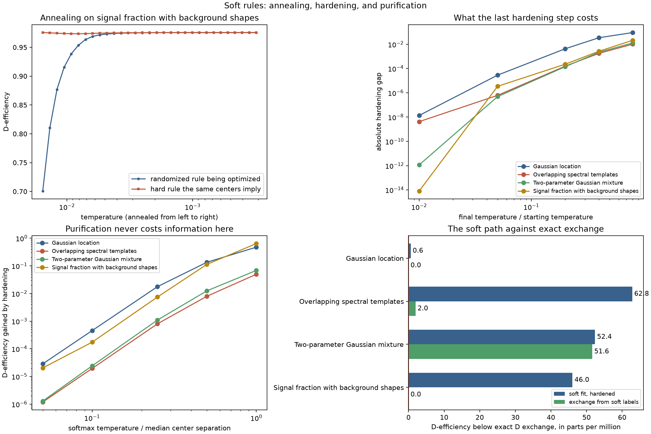
That distinction is not pedantic. The soft curve climbs enormously over the schedule while the hard curve barely moves, because at a high temperature the responsibilities are deliberately diffuse and every cell mean is pulled toward the global mean.

assert soft[0] < 0.9 < soft[-1]
assert abs(hard[-1] - hard[0]) < 0.05 * (soft[-1] - soft[0])

The hardening gap¶

A soft fit is never the deliverable: predict_scores assigns each score to its nearest center, which is the \(\tau\to0\) limit. The number that matters is the retention of that rule, and QuantizerResult.hardening_gap reports the difference,

\[\text{hardening gap} \;=\; (\text{soft retention at the last step}) - (\text{hard retention of the same centers}).\]

Cooling further closes it, which is what a temperature schedule is for.

gaps = []
for ratio in (0.5, 0.2, 0.05):
    annealed = sq.fit_quantizer(
        source,
        n_bins=n_bins,
        criterion=sq.DOptimality(),
        config=sq.SoftVoronoiConfig(
            seed=3,
            initializer_restarts=4,
            max_steps=120,
            record_every=120,
            temperature_end_ratio=ratio,
        ),
    )
    gaps.append(float(annealed.hardening_gap))

assert all(gap < 0.0 for gap in gaps)
assert all(abs(later) < abs(earlier) for earlier, later in zip(gaps, gaps[1:]))

Every gap here is negative: the hard rule retains more than the randomized rule that produced it. That is not a guarantee and the library does not treat it as one — it reports the number precisely because neither sign is forced.

Purification, measured¶

The negative sign above is a hint at something classical. If randomization could beat determinism, the soft relaxation would not be a computational device but a genuinely larger class of answers. For a population score law with no atoms it cannot: the Dvoretzky–Wald–Wolfowitz elimination-of-randomization theorem says every randomized \(K\)-action rule can be replaced by a deterministic one reproducing all \((W_b,m_b)\) exactly, and every criterion in this library depends on a rule only through those moments.

That theorem is an existence statement about an atomless law, and a finite sample is atomic by construction, so it does not cover the operation the library performs. What can be done is to measure the operation. Build genuinely randomized rules at several temperatures around the fitted centers, and compare each one against the deterministic rule obtained by taking every row's most probable cell.

The randomized side uses fractional_fisher_information, which is public and validates that the rows really are probability vectors. Turning it into the same D-efficiency number information_report publishes is one line of algebra, and the way to trust that line is to check it against a one-hot responsibility matrix, where both must agree exactly.

from examples.soft_purification import (
    center_separation,
    fractional_retention,
    hard_retention,
    softmax_responsibilities,
)

labels = np.asarray(rule.predict_scores(train.scores))
one_hot = np.eye(n_bins)[labels]

assert (
    abs(
        fractional_retention(train.scores, one_hot, train.weights)
        - hard_retention(train.scores, labels, train.weights, n_bins)
    )
    < 1e-12
)

With the helper grounded, the probe itself is short.

coordinates = np.asarray(rule.transform.apply(train.scores))
centers = np.asarray(rule.centers)
separation = center_separation(centers)

gains = []
for ratio in (1.0, 0.25):
    responsibilities = softmax_responsibilities(coordinates, centers, ratio * separation)
    randomized = fractional_retention(train.scores, responsibilities, train.weights)
    purified = hard_retention(
        train.scores, np.argmax(responsibilities, axis=1), train.weights, n_bins
    )
    gains.append(purified - randomized)

assert all(gain > 0.0 for gain in gains)
assert gains[0] > gains[1]

Hardening never cost information anywhere in this study, and at a temperature equal to the median center separation it gained a great deal. Read that as evidence consistent with purification, not as a proof of it on a finite table.

Against exact exchange¶

The soft path is one of several solvers for the same criterion, so the last question is simply whether it wins. Exact positive-gain exchange optimizes the hard objective directly; it can also be started from the soft fit's own labels.

exchange = sq.optimize_partition(
    train.scores, weights=train.weights, n_bins=n_bins, config=sq.DExchangeConfig(seed=3)
)
from_soft = sq.optimize_partition(
    train.scores,
    weights=train.weights,
    n_bins=n_bins,
    config=sq.DExchangeConfig(seed=3),
    initial_labels=labels,
)

soft_retention = float(rule.train_report.geometric_mean_retention)
assert exchange.train_report.geometric_mean_retention >= soft_retention - 1e-9
assert from_soft.train_report.geometric_mean_retention >= soft_retention - 1e-9

Analysis¶

Full-study numbers on 4000 training events, regenerated by examples/soft_purification.py into assets/soft-purification.json.

The schedule moves the soft objective, not the rule¶

The traced fit is the signal-plus-backgrounds problem at six cells, 300 Adam steps, cooling to one fiftieth of the starting temperature.

Quantity	At the first recorded step	At the last
Randomized rule (soft retention)	0.70076	0.97552
Hard rule the same centers imply	0.97557	0.97552

The soft objective climbs 27 D-efficiency points. The rule that will be deployed falls by 0.000046 — three hundred annealed gradient steps ended fractionally below the weighted k-means labeling they started from. Nothing is wrong: the optimizer maximized what it was given, which was the randomized objective at a nonzero temperature, and only in the \(\tau\to0\) limit are the two the same function. But it is a clean demonstration of why train_hard_retention exists and why watching trace.objective climb is not evidence of anything you can ship.

The hardening gap across problems and temperatures¶

The gap, as a function of the final temperature, on all four problems:

\(\tau_{\text{end}}/\tau_0\)	Gaussian location	Spectral templates	Gaussian mixture	Signal + backgrounds
0.8	-9.2e-02	-1.0e-02	-1.3e-02	-2.1e-02
0.4	-3.5e-02	-1.8e-03	-2.2e-03	-2.7e-03
0.2	-4.3e-03	-1.6e-04	-1.4e-04	-2.3e-04
0.05	-2.9e-05	-6.2e-07	-4.9e-07	-3.4e-06
0.01	-1.4e-08	-4.2e-09	-1.2e-12	+8.1e-15

Every entry above the level of floating-point noise is negative, so on these four problems hardening never lost information and usually gained a little. The gap closes by six or more orders of magnitude as the final temperature falls by a factor of eighty, which is a strong argument for the library's default temperature_end_ratio=0.05 and against reading anything into a fit that stopped warm. The single positive entry, \(+8\times10^{-15}\) at the coldest schedule, is a rounding difference between two nearly identical numbers; its sign carries no information.

assert sq.SoftVoronoiConfig().temperature_end_ratio == 0.05

Purification: what randomization costs¶

D-efficiency of a randomized rule against the deterministic rule that hardens it, at the same centers, with the softmax temperature written as a multiple of the median nearest-center separation:

\(\tau\) / separation	Randomized	Purified	Gain
1.00	0.33641	0.97552	0.639
0.50	0.86238	0.97552	0.113
0.25	0.96805	0.97552	0.00747
0.10	0.97535	0.97552	0.000174
0.05	0.97550	0.97552	0.0000204

Those are the signal-plus-backgrounds rows; the other three problems behave the same way, with gains that are positive at every temperature and every problem, ranging from 0.64 down to \(1.2\times10^{-6}\). At a temperature comparable to the cell spacing a randomized rule is catastrophically worse — it retains a third of the information the same centers retain when used deterministically — and the gap vanishes as the rule becomes deterministic.

This is what the classical result predicts and it is worth being precise about what has and has not been shown. Purification says a deterministic rule matching the randomized moments exists for an atomless law. The measurement above says that one specific deterministic rule — the argmax of these particular responsibilities — is never worse here. The second statement does not follow from the first, and on an atomic score law whether randomization can ever strictly help is open.

Soft against exchange¶

The same four problems, solved by the soft path, by exact exchange, and by exact exchange started from the soft fit's labels:

Problem	Cells	Soft, hardened	Exact D exchange	Exchange from soft labels
Gaussian location	4	0.8851049	0.8851055	0.8851055
Overlapping spectral templates	8	0.9968710	0.9969338	0.9969318
Two-parameter Gaussian mixture	8	0.9964000	0.9964524	0.9964008
Signal fraction with background shapes	6	0.9755215	0.9755675	0.9755675

Exact exchange wins on all four, by between 0.6 and 63 parts per million. Seeding exchange with the soft labels recovers the exchange answer on two problems and lands slightly below it on the other two, because a soft solution is a perfectly good exchange-stable point and exchange, being a local search, stops at the first one it cannot improve.

So the soft path is not a winner on retention here, and this page will not pretend otherwise. What it is, is the only route to two things exchange cannot do. It fits families that are not free labelings at all, which is what makes a rule rather than a labeling. And it accepts ProfiledDOptimality, where the exchange solver's result has no canonical compilation — the reusable profiled rule on the nuisance-profiled-ds page is exactly this solver, and there is no alternative to it.

Discussion¶

Task: space quantization (fit_quantizer), with optimize_partition appearing only as the comparison. Door: 1, precomputed score events. Criterion and solver: DOptimality with SoftVoronoiConfig throughout, against DExchangeConfig for the comparison; SoftVoronoiConfig also accepts ProfiledDOptimality, which is where it becomes indispensable rather than optional.

What the baselines did. The canonical baselines are not rerun here — the solver shootout already places soft gradient descent among the information-aware solvers, all of which beat a rectangular observation grid by six to thirty D-efficiency points. The comparison this page needs is internal: soft against hard, and randomized against deterministic.

What to take away. Cool the schedule, and judge the fit by train_hard_retention and hardening_gap rather than by the soft objective, which can climb 27 points while the deployed rule goes nowhere. Expect hardening to be free or slightly profitable, but check rather than assume — the library reports the number for that reason. And reach for the soft path when you need a rule under a criterion that has no compile bridge, not because it optimizes better than exact exchange, because on these problems it does not.

The matching notebook, soft_purification.ipynb, runs the full-size study, prints every table above, and re-renders the figure.