Door 2: mixture densities to a binned fraction measurement

This page solves space quantization (fit_quantizer) through Door 2: a linear-component model built from exact component pdfs. It absorbs the old "linear components" tutorial, and goes one step further: it fits from a bounded IntegrationSource end to end with two score columns, then measures what binning actually cost the downstream mixture-fraction estimate — not just the overall D-efficiency, but the retained Fisher information about the fraction specifically.

Problem

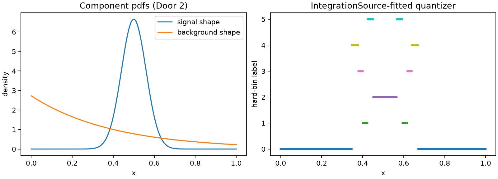
A one-dimensional spectrum is a mixture of a narrow signal peak and a broader truncated-exponential background, \(\lambda(x;c)=c_{\text{sig}}\phi_{\text{sig}}(x) + c_{\text{bkg}}\phi_{\text{bkg}}(x)\), with both \(\phi\) exact, normalized densities on \([0,1]\) and \(c_{\text{sig}}+c_{\text{bkg}}=1\). The event score at the reference coefficients is \(s_k(x)=\phi_k(x)/\lambda(x;c_0)\) — scores_from_components's exact identity. c_sig is the parameter of interest (the mixture fraction); c_bkg is a nuisance shape parameter here treated jointly, so every fit below is plain DOptimality on both columns together.

Data

examples.synthetic_problems.signal_background_shape returns the exact densities and precomputed Monte Carlo splits. One background shape keeps this a clean two-parameter problem — exactly the case an IntegrationSource must handle correctly.

import numpy as np

import scorequant as sq
from examples.synthetic_problems import signal_background_shape

problem = signal_background_shape(background_rates=(2.5,), n_bins=6)
problem.component_names, problem.interest, problem.nuisance, problem.coefficients

The component pdfs are exact callables; wrapping them as LinearComponents makes the "component pdfs → score" step an explicit API call rather than something the generator did silently.

def signal_component(x):
    return problem.signal_density(np.asarray(x)[:, 0])


def background_component(x):
    return problem.background_densities[0](np.asarray(x)[:, 0])


model = sq.LinearComponents(
    components={"signal": signal_component, "background": background_component},
    coefficients={
        "signal": float(problem.coefficients[0]),
        "background": float(problem.coefficients[1]),
    },
    variables=["x"],
)
provider = sq.LinearComponentScore(model)

reproduced = np.asarray(provider.score(problem.train.observations))
assert np.allclose(reproduced, problem.train.scores)

API walkthrough

Fit from a Monte Carlo observation sample

The generator's Monte Carlo splits pair physical observations with the reference intensity as their weight, so ObservationSample plus provider reaches fit_quantizer directly.

train, test = problem.train, problem.test
assert train.observations.shape == (4000, 1)

quantizer_mc = sq.fit_quantizer(
    sq.ObservationSample(train.observations, train.weights),
    provider=provider,
    n_bins=problem.n_bins,
    criterion=sq.DOptimality(),
    config=sq.DExchangeConfig(seed=50),
)
mc_retention = float(
    quantizer_mc.evaluate_scores(test.scores, test.weights).geometric_mean_retention
)
assert 0.99 < mc_retention <= 1.0

Fit from a bounded IntegrationSource, end to end

The density is bounded on [0, 1] and exact, so no Monte Carlo sample is needed at all: a deterministic Gauss-Legendre grid over problem.bounds, weighted by the mixture density, is the whole reference measure. This is the required two-parameter IntegrationSource path — provider returns one score column per component, so this run carries two.

source = sq.IntegrationSource(
    problem.bounds, density=problem.intensity, quadrature=sq.GaussLegendreConfig(order=64)
)
quantizer_int = sq.fit_quantizer(
    source,
    provider=provider,
    n_bins=problem.n_bins,
    criterion=sq.DOptimality(),
    config=sq.DExchangeConfig(seed=50),
)
assert quantizer_int.source_kind == "integration_source"
assert quantizer_int.transform.rank == 2
int_retention = float(
    quantizer_int.evaluate_scores(test.scores, test.weights).geometric_mean_retention
)
assert 0.99 < int_retention <= 1.0
assert round(mc_retention, 4) == round(int_retention, 4)

The two fits — one from a 4000-event Monte Carlo sample, one from a 64-point deterministic quadrature grid — land on the same held-out D-efficiency to four decimal places. For a low-dimensional bounded model, IntegrationSource gets the exact reference measure without paying for a Monte Carlo sample at all.

Analysis: the downstream payoff

The overall D-efficiency above compresses both coefficients jointly. The question that actually matters for a mixture-fraction measurement is narrower: how much information about c_sig specifically survived the six bins? profiled_information_report answers this for any labels, independent of what criterion produced them, by Schur-completing the nuisance block out of both the unbinned and the binned Fisher matrix.

labels = np.asarray(quantizer_int.predict_scores(test.scores))
profiled = sq.profiled_information_report(
    test.scores, labels, interest=problem.interest, weights=test.weights, n_bins=problem.n_bins
)
fraction_retention = float(profiled.geometric_mean_retention)
assert round(fraction_retention, 3) == 0.996
schur_ratio = float(profiled.schur_binned[0, 0] / profiled.schur_unbinned[0, 0])
assert 0.99 < schur_ratio < 1.0  # strictly less than the unbinned ceiling

Six bins retain about 99.6% of the Fisher information specifically about the signal fraction — close to, but strictly less than, the unbinned ceiling. That gap is exactly what a binned mixture-fraction fit pays for compression; profiled.schur_unbinned and profiled.schur_binned are the two \(1\times1\) matrices a downstream likelihood's asymptotic variance would use.

Discussion

Task: space quantization (fit_quantizer). Door: 2, an analytic component model — both an ObservationSample Monte Carlo route and the required IntegrationSource route with two score columns. Criterion / solver: DOptimality with exact exchange throughout; profiled_information_report is applied afterward as a diagnostic and does not need to be the fitting criterion.

This page treats c_sig and c_bkg jointly rather than fitting with ProfiledDOptimality. When the background shape is a genuine nuisance you want optimized around rather than just reported on, that is a different, deliberate choice of criterion — see Chapter 10 and a later profiled-\(D_s\) page for the deeper D-versus-profiled-D comparison this same generator was built for.

The matching notebook, door2_mixture_densities.ipynb, runs both fits at full sample size and inspects the retained Fisher matrix directly.