The FlowCyt study

Flow cytometry produces a cloud of cells, not a row of population fractions. Each cell carries twelve marker measurements. The practical result, however, is often only six numbers: the proportions of T cells, B cells, monocytes, mast cells, hematopoietic stem/progenitor cells (HSPCs), and everything else.

This study asks a deliberately hard compression question:

Can we replace 200,000 held-out twelve-dimensional test events with a few integer bin counts and still recover the population fractions?

The answer on the frozen FlowCyt experiment is yes. The operating point uses eight learned hard bins. Eight bins retain 98.5% of the supplied-score surrogate information and reach 0.00193 macro RMSE on the ten held-out patients. The selected unbinned classifier-ratio baseline is slightly better at 0.00173 RMSE, as the exact-information ordering suggests it should be when ratio bias is sufficiently controlled.

Those numbers are not fixture results. They come from all 30 FlowCyt patients, with 20 reference patients and ten frozen held-out test patients. The reproducible bounded study contains 600,000 real cells sampled from 21,254,866 upstream events.

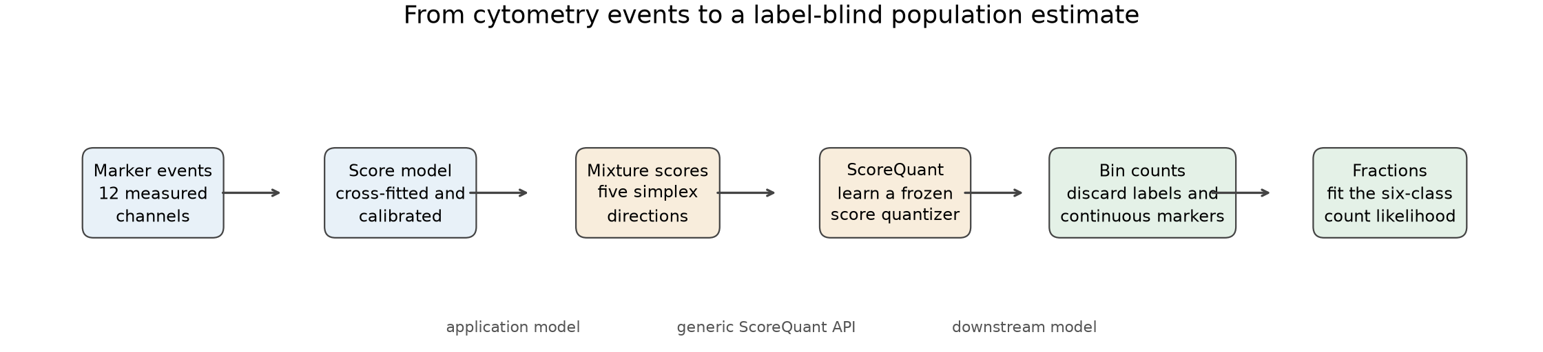
The important boundary is visible in the figure. The classifier is not ScoreQuant. Neither is the downstream mixture likelihood. ScoreQuant receives score vectors and returns a frozen score quantizer. This makes the study useful for cytometry users and for developers adapting the same API to another domain.

The section

Page	What it settles
Problem and data	The benchmark, its licence, the bounded 600,000-cell acquisition protocol, the frozen patient split, the committed CI fixture, and the full-corpus transport audit
Score model and calibration	How twelve markers become five mixture-score coordinates, the nested calibration audit that chose the ratio model, and what the normalization residual does and does not prove
Quantization at scale	The zero-configuration fit_quantizer call on 600,000 cells, retention against bin budget, the finite-D exchange and its compile bridge, the downstream mixture fit, uncertainty, and transport diagnostics
One fraction of interest	What changes when the measurement is a single population fraction with the rest of the composition floating: plain D against profiled \(D_s\), a certified ceiling, and the downstream interval
Solver comparison	Every applicable solver and the three canonical baselines, at both the frozen fixture and the 600,000-cell sample: train and held-out retention, search effort, and wall-clock cost

Result at a glance

The predeclared acceptance gate required learned score partitions to beat the median random score partition in held-out D-efficiency for at least five of six bin counts, and to be no worse than marker k-means in population RMSE for at least four. The result was 6/6 for both tests.

Bins	Soft Voronoi RMSE	Score k-means RMSE	Marker k-means RMSE	Random RMSE median	Supplied-score D-efficiency	Random D-efficiency median
5	0.03000	0.00501	0.04186	0.02998	0.391	0.001
8	0.00193	0.00209	0.02889	0.01870	0.985	0.016
10	0.00202	0.00206	0.04758	0.01147	0.990	0.060
15	0.00204	0.00217	0.03332	0.01046	0.995	0.099
20	0.00212	0.00243	0.03220	0.00730	0.996	0.260
30	0.00260	0.00280	0.04990	0.00697	0.998	0.324

Every number on this page comes from the committed evidence, not from prose.

import json
from pathlib import Path

metrics = json.loads(Path("docs/usecases/assets/cell_population.json").read_text())

assert metrics["source"]["sample_rows"] == 600_000
assert metrics["run"]["quick"] is False
assert metrics["acceptance"]["random_d_efficiency_wins"] == 6
assert metrics["acceptance"]["marker_rmse_noninferiority_wins"] == 6

eight = metrics["soft_voronoi:8"]
assert round(eight["target_macro_rmse"], 5) == 0.00193
assert round(eight["held_out_d_efficiency"], 3) == 0.985
assert round(metrics["unbinned_classifier_ratio"]["target_macro_rmse"], 5) == 0.00173

Eight bins are the useful knee in this experiment and give the lowest learned- partition RMSE. Five bins are an explicit negative result, but not an optimizer mystery: they cannot identify five independent fractions from a fixed-total count likelihood, which Quantization at scale proves. Thirty bins preserve more local supplied-score information but contain an empty held-out bin and do not improve the downstream estimate. More bins are not automatically better, and the hard result — not the soft objective — is what matters.

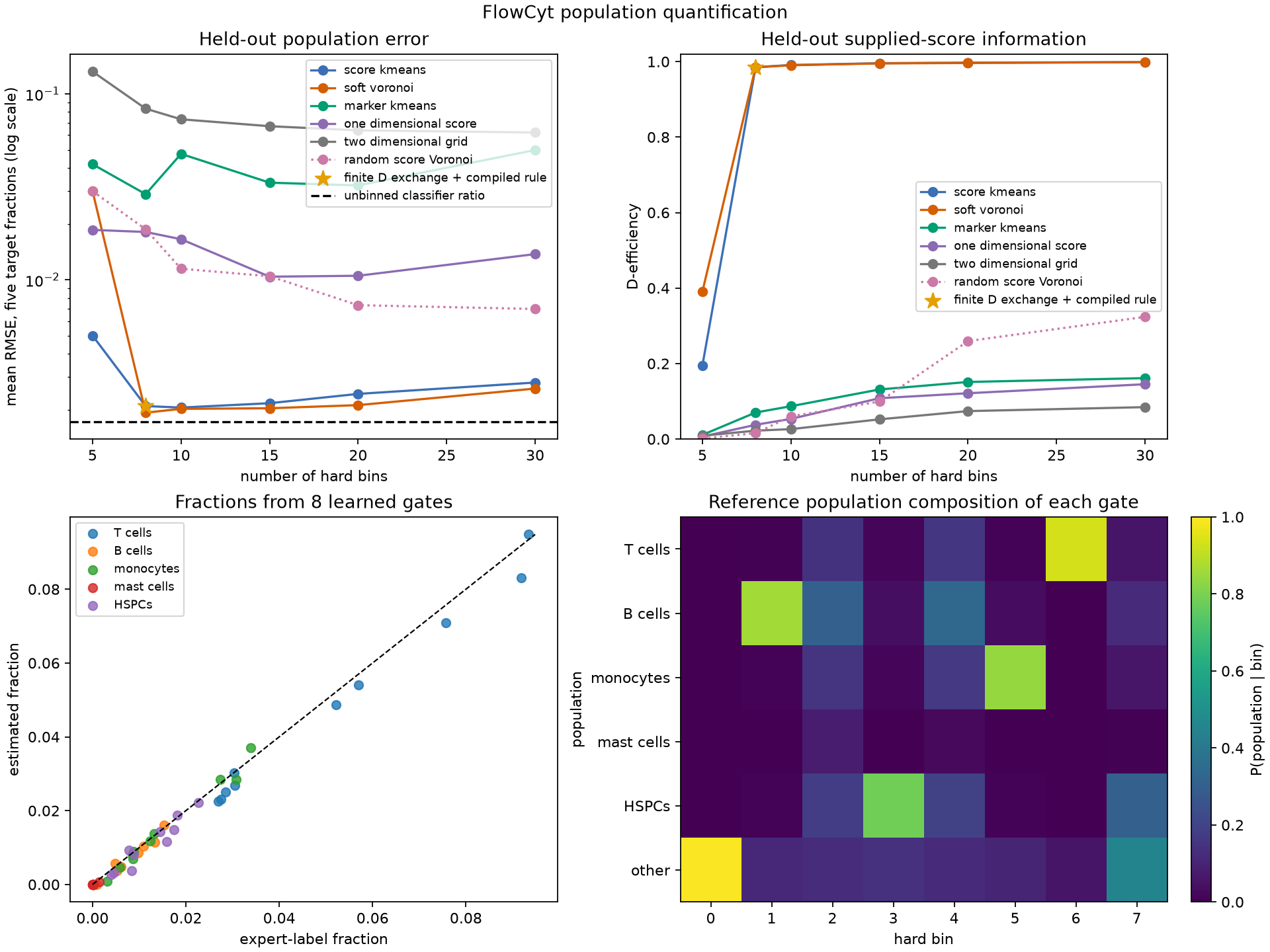
The lower-left panel shows each estimated target fraction against the expert fraction for the ten test patients. The lower-right panel does not project the five-dimensional partition. It shows \(P(k\mid B_j,\theta_0)\), the reference population composition of each of the eight gates. This projection-free summary explains the statistical role of each gate.

The complete numeric record is committed as cell_population.json. It includes every method/bin result, per-patient estimates, calibration and shift diagnostics, reference-only closure and uncertainty coverage, run settings, timings, source provenance, and acceptance decisions. The profiled-\(D_s\) extension keeps its own evidence in flowcyt_profiled_ds.json.

What this study establishes

On this frozen all-patient sample, a handful of score-aware hard gates preserve the parameter information that ordinary marker-space partitions miss. Eight bins are already enough for a practical result. The study also shows the limits clearly: score calibration matters, fixed-total identifiability must be checked separately from an intensity-information objective, high information retention does not prevent empty transported bins, local Fisher errors fail for fractions on the simplex boundary, and — as the profiled extension shows — a criterion aimed at one fraction can be worth almost nothing once plain D is already close to a certified ceiling.

That combination is the useful result. ScoreQuant is not a classifier and not a mixture fitter. It is the compression layer between them, and this case shows how to build, test, diagnose, and reproduce that layer on real data.