2. One dimension by hand
Before any of this becomes a matrix problem, it is worth solving the smallest interesting case completely, with a pencil. One parameter, one score coordinate, two cells. The answer is a number you can remember — \(2/\pi\) — and the way it is derived contains, in miniature, every structural idea the rest of the book generalizes.
The problem is also old. Cox (1957) asked exactly this question under the name "grouping": if a normal sample must be reported as counts in \(K\) groups, where should the group boundaries go so that as little information about the mean as possible is lost? Six years earlier Ogawa (1951) had studied the asymptotic version, choosing spacings of order statistics to maximize retained Fisher information. What follows is their problem, in the language this book will use for the multivariate case.
The model
Let \(X \sim \mathcal{N}(\theta, 1)\) and take the reference point \(\theta_0 = 0\). Then
The score map is the identity, so the score law is the standard normal \(P_S = \mathcal{N}(0,1)\) and the unbinned information is \(I_{\text{full}} = \mathbb{E}[S^2] = 1\). Every retention number below is therefore just \(I_q\) itself.
Two facts do all the work. First, the information carried by a hard label is the variance of the conditional score mean,
Chapter 5 derives this in full generality; the intuition is that a count in cell \(b\) tells you only that \(S\) landed there, so the derivative of its log probability with respect to \(\theta\) is the average score of the events inside. Second, conditioning splits the second moment,
with no centering anywhere: both sides are uncentered second moments. In one dimension this identity has a striking consequence. Since \(I_{\text{full}}\) does not depend on the rule, maximizing the retained information is exactly minimizing the mean squared within-cell error — the classical objective of scalar quantizer design. Chapter 3 cashes that equivalence in. It is special to one dimension: once the criterion is \(\log\det I_q\) on a matrix, no such reduction survives.
Two cells
Consider the threshold rule \(q_t(s) = \mathbf{1}\{s > t\}\). Because \(\frac{d}{ds}\big[-\varphi(s)\big] = s\,\varphi(s)\), the cell moments are available in closed form:
and therefore, using \(I_q = \sum_b m_b^2 / W_b\),
Where does the optimum sit? The first-order condition for an interior boundary is that neither neighboring cell is more attractive than the other — in one dimension, that the boundary lies at the midpoint of the two conditional means, \(t = \tfrac12(\mu_-+\mu_+)\). By symmetry of the standard normal \(\mu_- = -\mu_+\), so \(t=0\) satisfies it. The standard normal density is log-concave, which is the classical condition under which this stationary rule is unique, so the symmetric split is the optimum and not merely a critical point. Differentiating directly gives the same picture,
which vanishes at \(t=0\) and is negative for every \(t>0\).
Now evaluate. At \(t=0\) the two cells have equal probability \(W_\pm = 1/2\), and the conditional mean of the positive half is the mean of a half-normal:
Hence
A single yes/no answer about a Gaussian observation preserves \(2/\pi\) of its Fisher information — and the mnemonic is that the retained information is the square of the mean absolute deviation. The complementary loss is \(1 - 2/\pi \approx 0.3634\), and standard errors inflate by \(\sqrt{\pi/2} \approx 1.2533\), which is the number Chapter 1 measured by brute force.
Two properties of this answer are worth pausing on. It does not depend on \(\theta_0\) or on the variance: rescaling the score rescales \(I_q\) and \(I_{\text{full}}\) together. And it depends on the sign of \(s\) only, never on the magnitude — which is precisely why one bit is so expensive.
Checking the algebra
The closed form first, at machine precision, and then the same statement through the library on a sample.
import math

import numpy as np

import scorequant as sq


def normal_pdf(x):
    """Standard normal density."""
    return np.exp(-0.5 * np.asarray(x, dtype=float) ** 2) / math.sqrt(2.0 * math.pi)


def normal_cdf(x):
    """Standard normal distribution function."""
    return 0.5 * (1.0 + np.vectorize(math.erf)(np.asarray(x, dtype=float) / math.sqrt(2.0)))


def two_cell_information(t):
    """Information kept by the rule that reports whether the score exceeds t."""
    return normal_pdf(t) ** 2 / (normal_cdf(t) * (1.0 - normal_cdf(t)))


assert abs(float(two_cell_information(0.0)) - 2.0 / math.pi) < 1e-12

sweep = np.linspace(-2.5, 2.5, 5_001)
values = two_cell_information(sweep)
assert abs(sweep[int(np.argmax(values))]) < 1e-9
assert values.max() <= 2.0 / math.pi + 1e-12
The sweep confirms that the symmetric split is the maximum and that nothing beats \(2/\pi\). Now the empirical side: draw a sample, split it at zero, and ask the library what the labels retained.
rng = np.random.default_rng(0)
scores = rng.normal(size=(20_000, 1))

hand_labels = (scores[:, 0] > 0.0).astype(int)
report = sq.information_report(scores, hand_labels, n_bins=2)
retention = float(report.geometric_mean_retention)

assert abs(retention - 2.0 / math.pi) < 0.02
print(round(retention, 4), round(2.0 / math.pi, 4))
The reported number is the retained fraction defined in Chapter 1; with a single score coordinate it is exactly \(I_q/I_{\text{full}}\), and it lands on \(2/\pi\) up to sampling noise.
The population optimum is not the sample optimum
The threshold \(t=0\) is optimal for the law. It is not, in general, optimal for a particular finite sample drawn from that law — the empirical cell means are not exactly \(\pm\sqrt{2/\pi}\), so the empirical midpoint is not exactly zero. ScoreQuant can be asked directly whether any single event would rather be in the other cell.
sample = rng.normal(size=(4_000, 1))
split_at_zero = (sample[:, 0] > 0.0).astype(int)

stability = sq.exchange_stability_report(sample, split_at_zero, criterion=sq.DOptimality())
assert stability.best_gain < 1e-3

exact = sq.fit_quantizer(
    sq.ScoreSample(sample),
    n_bins=2,
    criterion=sq.DOptimality(),
    config=sq.ScalarDPConfig(),
)
labels = np.asarray(exact.labels)
lower = sample[labels == labels[np.argmin(sample[:, 0])], 0].max()
upper = sample[labels != labels[np.argmin(sample[:, 0])], 0].min()
sample_boundary = 0.5 * (lower + upper)

hand_on_sample = sq.information_report(sample, split_at_zero, n_bins=2)
assert abs(sample_boundary) < 0.1
assert exact.train_report.geometric_mean_retention >= hand_on_sample.geometric_mean_retention
print(round(stability.best_gain, 8), round(float(sample_boundary), 4))
The best available single-event relocation is worth a few millionths of a nat, and the exactly optimal sample boundary sits within a hundredth of the origin. The distinction is negligible here and it will not always be. Chapter 6 gives it a name and Chapter 8 shows that for the determinant criterion the two problems are joined by a theorem rather than by an approximation.
More than two cells
The midpoint condition generalizes immediately. With cells \((-\infty,t_1],\,(t_1,t_2],\dots,(t_{K-1},\infty)\), a stationary rule satisfies
with the conventions \(t_0 = -\infty\), \(t_K = +\infty\). Iterating the two lines to a fixed point is a handful of numpy, and it converges from the equal-frequency starting point.
def equal_frequency_thresholds(n_bins):
    """Cut points that give every cell the same probability."""
    grid = np.linspace(-8.0, 8.0, 200_001)
    return np.interp(np.arange(1, n_bins) / n_bins, normal_cdf(grid), grid)


def retained_information(thresholds):
    """Information kept by an interval rule with the given interior cut points."""
    edges = np.concatenate(([-np.inf], np.asarray(thresholds, dtype=float), [np.inf]))
    cell_weights = normal_cdf(edges[1:]) - normal_cdf(edges[:-1])
    cell_moments = normal_pdf(edges[:-1]) - normal_pdf(edges[1:])
    return float(np.sum(cell_moments**2 / cell_weights))


def optimal_thresholds(n_bins, iterations=2_000):
    """Iterate the midpoint condition from equal-frequency cut points."""
    thresholds = equal_frequency_thresholds(n_bins)
    for _ in range(iterations):
        edges = np.concatenate(([-np.inf], thresholds, [np.inf]))
        cell_weights = normal_cdf(edges[1:]) - normal_cdf(edges[:-1])
        cell_means = (normal_pdf(edges[:-1]) - normal_pdf(edges[1:])) / cell_weights
        thresholds = 0.5 * (cell_means[:-1] + cell_means[1:])
    return thresholds


best = {k: retained_information(optimal_thresholds(k)) for k in range(2, 9)}
equal = {k: retained_information(equal_frequency_thresholds(k)) for k in range(2, 9)}

assert abs(best[2] - 2.0 / math.pi) < 1e-10
assert abs(best[2] - equal[2]) < 1e-9  # the median is the optimal two-cell split
assert all(best[k] >= equal[k] - 1e-12 for k in best)
assert all(best[k] < best[k + 1] for k in range(2, 8))
for k in best:
    print(k, round(best[k], 6), round(equal[k], 6))
| cells \(K\) | optimal edges | equal-frequency edges |
|---|---|---|
| 2 | 0.636620 | 0.636620 |
| 3 | 0.809826 | 0.793229 |
| 4 | 0.882518 | 0.860559 |
| 5 | 0.920059 | 0.896955 |
| 6 | 0.942022 | 0.919361 |
| 7 | 0.956000 | 0.934368 |
| 8 | 0.965452 | 0.945034 |
The first column is the classical grouping efficiency of a normal location parameter. Three cells already recover 81%, eight recover 96.5%. The second column is what you get from the reflex of putting an equal number of events in every bin: never better, and by \(K=8\) it is throwing away about two extra percentage points of information — roughly the equivalent of discarding one event in fifty.
The reason is visible in the optimal cut points. For eight cells they are \(0, \pm0.5005, \pm1.0500, \pm1.7479\), while equal frequency puts them at \(0, \pm0.3186, \pm0.6745, \pm1.1503\). The information-optimal rule pushes its boundaries outward, spending resolution on the tails. That is not a quirk: the quantity being resolved is the score, and in the tails the score is large, so a misplaced boundary there costs far more than a misplaced boundary in the crowded center. Equal frequency optimizes occupancy; nobody asked for occupancy.
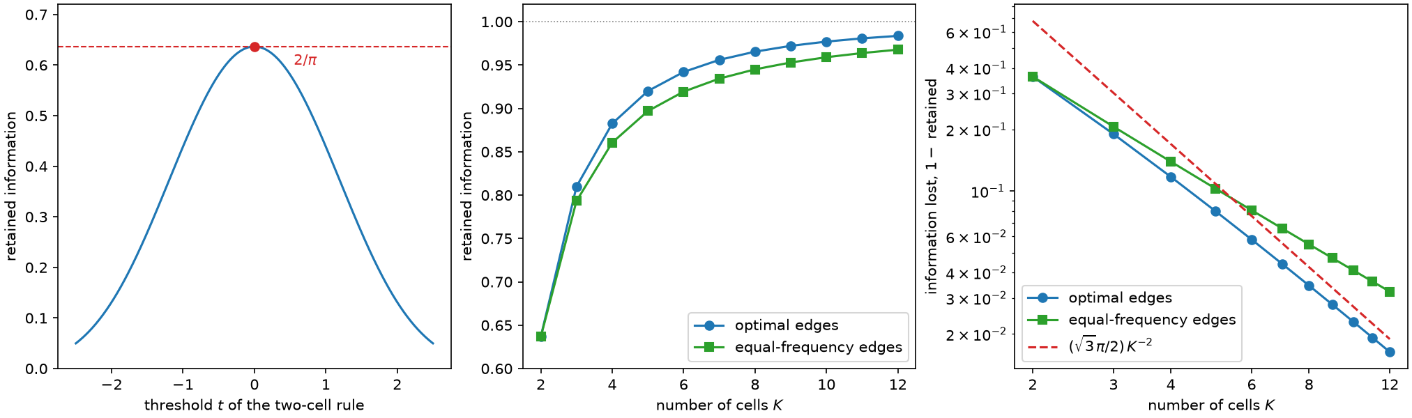
Left: information kept by a two-cell rule as a function of its threshold, peaking at \(2/\pi\) for the symmetric split. Middle: retained information against the number of cells, for optimal and for equal-frequency edges. Right: the same loss on logarithmic axes, against the high-resolution reference \((\sqrt3\pi/2)K^{-2}\).
How fast does the loss vanish?
The right-hand panel answers the natural follow-up. Because in one dimension retained information is one minus the mean squared quantization error of the score, the classical high-resolution theory applies verbatim: for a smooth density the optimal \(K\)-cell loss behaves like \(\tfrac{1}{12}\big(\int f^{1/3}\big)^3 K^{-2}\) in units of \(\mathbb{E}[S^2]\), which is one here, so for the standard normal the reference curve is \((\sqrt3\pi/2)\,K^{-2} \approx 2.72\,K^{-2}\). The approach is slow because Gaussian tails are long, but the exponent is already clear by \(K=12\).
Two practical consequences follow. Doubling the number of cells quarters the remaining loss, so the marginal value of a bin falls off a cliff — most of what there is to gain is gained by \(K\approx 6\). And the loss is a property of the score law: a heavy-tailed or multimodal score is far more expensive to quantize than a Gaussian one, which is exactly the situation Chapter 3 examines.
What generalizes and what does not
Three ideas from this chapter survive into the rest of the book. The information of a label is the variance of the conditional score mean. A stationary rule assigns each event to the nearest cell representative. And the boundaries follow the score, not the event count.
One idea does not survive. Here the criterion was a scalar, so "maximize retained information" and "minimize within-cell scatter" were the same instruction, and the optimum could be found by iterating a midpoint rule. With two or more parameters the criterion becomes a function of a matrix, the notion of "nearest" acquires a metric that depends on the current partition, and iterating the analogous rule can make the objective worse. That story starts in Chapter 5. First, though, Chapter 3 finishes the one-dimensional case properly: not a fixed point that might be local, but the exact global optimum.