Evidence gallery

Three synthetic problems, each fitted twice by ScoreQuant and three times by a naive alternative, all scored on an untouched test split. Every figure and every number on this page is regenerated deterministically by the matching script in examples/, and the numbers are read back from the committed JSON summaries next to the figures.

JAX_ENABLE_X64=1 MPLBACKEND=Agg uv run python -m examples.gaussian_location
JAX_ENABLE_X64=1 MPLBACKEND=Agg uv run python -m examples.spectral_templates
JAX_ENABLE_X64=1 MPLBACKEND=Agg uv run python -m examples.spatial_sources
JAX_ENABLE_X64=1 MPLBACKEND=Agg \
  uv run python -m examples.cell_population \
  --fixture examples/data/flowcyt_fixture.npz --quick

The headline metric is D-efficiency: the geometric mean of the retained-information eigenvalues, which lies between zero and one whenever the Fisher invariants hold. One means hard binning cost nothing; zero means a direction of the Fisher information was destroyed outright.

What the three problems stress

They are not three variations of one thing. Each isolates a different way a binning can go wrong.

Problem	Observation space	Score columns	Bins	What it stresses
Gaussian location	one dimension	1	4	The control case. The score is the observation, so score space and observation space coincide and no method should be able to beat any other by much.
Overlapping spectral templates	one dimension	2	8	Geometry. One observation coordinate folds onto a non-monotone score curve, so nearby observations can carry opposite information.
Overlapping spatial sources	two dimensions	2	16	Dimensionality and overlap. Four overlapping bumps in the plane, where an observation-space grid must spend cells on directions that carry no information.

Read across the three tables below and one pattern dominates: the two ScoreQuant fits agree with each other everywhere, while the observation-space baselines fall away exactly as the observation-to-score map stops being the identity. On the control problem the gap is 0.0001; on the spatial problem it is 0.07.

For a full method-by-method comparison on a single problem — every solver the library dispatches, the three canonical baselines, retention and cost — see the solver shootout.

The five methods in every table

Row	What it is
Whitened score k-means	fit_quantizer with NormalizedTrace and KMeansConfig
Soft Voronoi	fit_quantizer with DOptimality and SoftVoronoiConfig
Observation k-means	Baseline: weighted k-means on the raw observation coordinates
Equal-frequency observation grid	Baseline: quantile edges along each observation axis
Random score centers	Reference: the median of fifty random draws of n_bins training score rows used as centers

The equal-frequency grid here uses quantile edges, which is a slightly stronger baseline than the equal-width rectangular_observation_bins used on the solver-shootout page. The random-centers row is not a method anyone would use; it is the floor a method has to clear to have earned anything.

Each run also fits with a validation split. Those numbers are in the JSON files and are diagnostic only: they never influence gradients, stopping, or checkpoint selection.

Gaussian location

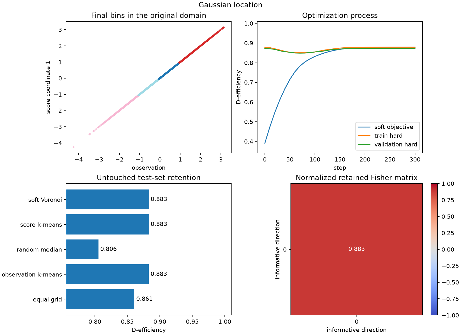
A standard normal observation with the analytic score \(s(x)=x\), compressed into four bins. Two thousand training and ten thousand held-out events.

Method	Train D-efficiency	Held-out D-efficiency
Whitened score k-means	0.87889	0.88327
Soft Voronoi	0.87889	0.88325
Observation k-means	0.87884	0.88314
Equal-frequency observation grid	0.85487	0.86104
Random score centers	0.80174	0.80573

This is the control, and it behaves like one. Observation k-means is within 0.0002 of the score-space fits, because here the observation is the score and clustering one is clustering the other. The 0.88 ceiling is not a failure of the optimizer: four hard bins on a one-dimensional Gaussian simply cannot retain everything, and the quantile grid gives away another two points on top of that.

Overlapping spectral templates

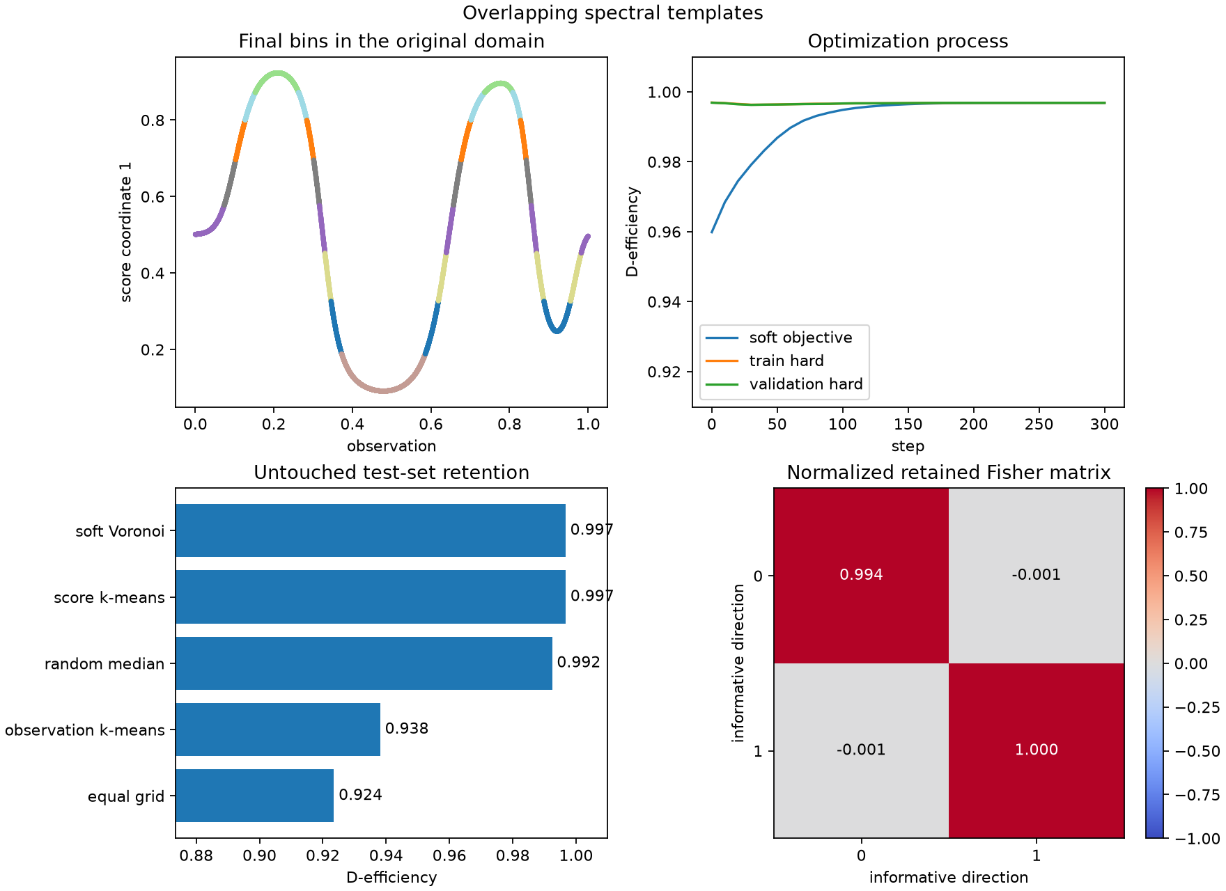
Two overlapping emission templates on \([0,1]\), weighted by the mixture intensity, with two exact component-score columns and eight bins. Four thousand training and fifteen thousand held-out events.

Method	Train D-efficiency	Held-out D-efficiency
Whitened score k-means	0.99693	0.99674
Soft Voronoi	0.99688	0.99669
Observation k-means	0.94106	0.93815
Equal-frequency observation grid	0.92842	0.92352
Random score centers	0.99277	0.99246

The score curve folds: the same score value is reached at two well-separated positions, so a bin that is contiguous in the observation coordinate is not contiguous in information. Observation k-means gives up almost six points to that fold. The striking row is the last one — random centers drawn in score space beat careful clustering in observation space by five points. Being in the right space matters more here than optimizing well within it.

Overlapping spatial sources

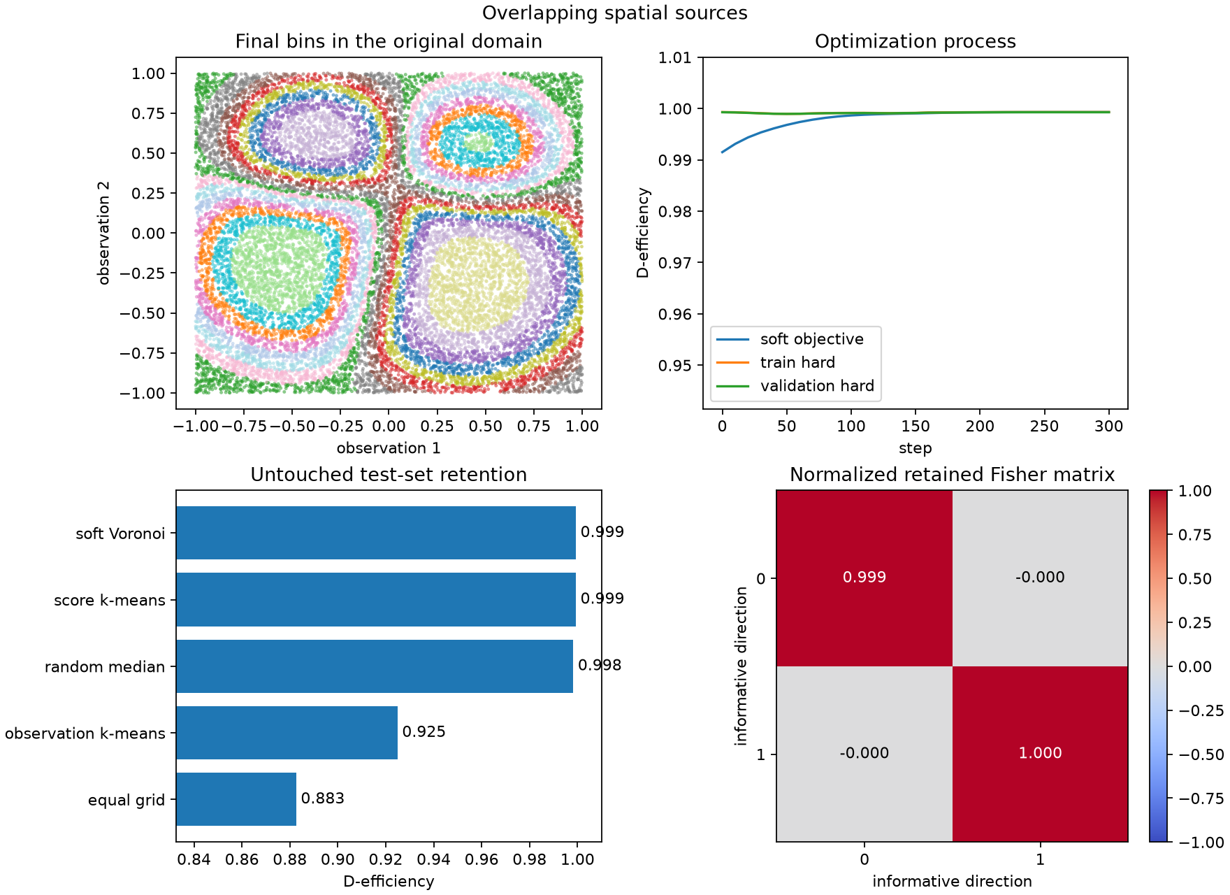
Two overlapping two-dimensional sources, each a pair of Gaussian bumps, importance-weighted by the mixture intensity and compressed into sixteen bins. Six thousand training and twenty thousand held-out events.

Method	Train D-efficiency	Held-out D-efficiency
Whitened score k-means	0.99930	0.99927
Soft Voronoi	0.99930	0.99927
Observation k-means	0.93118	0.92487
Equal-frequency observation grid	0.89099	0.88262
Random score centers	0.99816	0.99819

The score-space fits retain essentially everything, while the observation-space grid loses almost twelve points. In two dimensions a grid has to spend its cells on both axes whether or not both carry information, and here the informative structure is a pair of curved level sets that no axis-aligned rectangle follows.

The numbers on this page are checked

Every value in the three tables above is transcribed from the committed JSON summaries. The block below reads those files and fails if any transcription has drifted, so the prose cannot quietly diverge from the evidence.

import json
from pathlib import Path

import examples

GALLERY = Path(examples.__file__).resolve().parents[1] / "docs" / "gallery"

PUBLISHED = {
    "gaussian_location": {
        "kmeans": (0.87889, 0.88327),
        "soft": (0.87889, 0.88325),
        "observation_kmeans": (0.87884, 0.88314),
        "equal_grid": (0.85487, 0.86104),
        "random_median": (0.80174, 0.80573),
    },
    "spectral_templates": {
        "kmeans": (0.99693, 0.99674),
        "soft": (0.99688, 0.99669),
        "observation_kmeans": (0.94106, 0.93815),
        "equal_grid": (0.92842, 0.92352),
        "random_median": (0.99277, 0.99246),
    },
    "spatial_sources": {
        "kmeans": (0.99930, 0.99927),
        "soft": (0.99930, 0.99927),
        "observation_kmeans": (0.93118, 0.92487),
        "equal_grid": (0.89099, 0.88262),
        "random_median": (0.99816, 0.99819),
    },
}

for problem, rows in PUBLISHED.items():
    metrics = json.loads((GALLERY / f"{problem}.json").read_text(encoding="utf-8"))
    assert metrics["problem"] == problem
    for method, (train, held_out) in rows.items():
        assert round(metrics[f"{method}_train_retention"], 5) == train
        assert round(metrics[f"{method}_test_retention"], 5) == held_out

gaussian = json.loads((GALLERY / "gaussian_location.json").read_text(encoding="utf-8"))
spatial = json.loads((GALLERY / "spatial_sources.json").read_text(encoding="utf-8"))
control_gap = gaussian["kmeans_test_retention"] - gaussian["observation_kmeans_test_retention"]
spatial_gap = spatial["kmeans_test_retention"] - spatial["observation_kmeans_test_retention"]
assert round(control_gap, 4) == 0.0001
assert round(spatial_gap, 2) == 0.07

These runs establish exact information identities and empirical held-out behavior. They do not claim that either optimizer found a globally optimal partition; for that question see the certification machinery rather than this page.

FlowCyt cell-population quantification

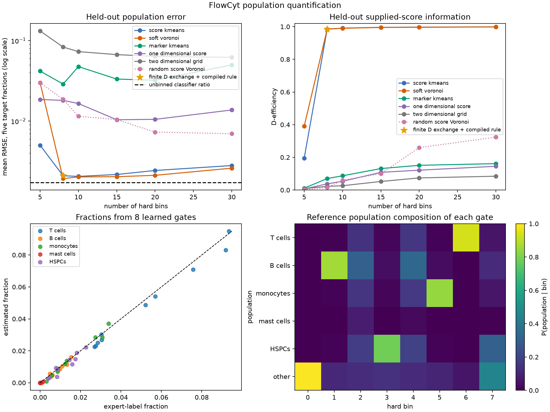
The complete FlowCyt study uses all 30 patients, 600,000 real cells, a frozen ten-patient test cohort, competing partitions, a downstream mixture likelihood, uncertainty checks, and machine-readable evidence. The cell_population command above is its small integration path; the page documents the reproducible all-patient run.