HEP classifier study: a tau-energy-scale nuisance from the FAIR Universe HiggsML dataset

This page is the reference study behind the portal's HEP walkthrough. It walks Door 3 (classifier to density ratios to scores) through profiled \(D_s\) on a real particle-physics dataset: the FAIR Universe HiggsML Uncertainty Challenge public sample, with an explicit tau-energy-scale (tes) nuisance. It is the project's only example that estimates a nuisance-shape score column through the library's central-difference door, CentralLogRatioScore, and the only one whose reusable rules are evaluated on events they never saw and carried through to a downstream signal-strength fit.

Everything here is a simulation study on a committed 1,000-event fixture, not a measurement.

The measurement

The model is an extended linear intensity over the fixture's events,

\[\lambda(x;\mu,\nu,\alpha)=\mu\,s(x;\alpha)+\nu\,b(x;\alpha),\]

with reference point \(\theta_0=(1,1,1)\) and three parameters: \(\mu\), the htautau signal rate (of interest); \(\nu\), the combined background rate (nuisance, normalization); and \(\alpha\), the tau energy scale tes (nuisance, shape).

The energy scale is unconstrained. Nothing in this study adds an external constraint on \(\alpha\): neither the profiled criterion, nor the profiled information any retention number divides by, nor the primary downstream uncertainty. A Gaussian constraint of width 0.01 is recorded next to the downstream number to show what a physical constraint would change (below: nothing, at this fixture's yields).

Why the backgrounds are collapsed. ztautau, ttbar, and diboson are collapsed into one background component. This is forced, not chosen: the committed sample carries 634 ztautau, 26 ttbar, and 4 diboson rows -- far too few of the latter two to support separate rate normalizations. A reader who knows the challenge will expect the three background normalizations upstream's systematics.py exposes; this study measures one combined background rate instead.

Data and provenance

The fixture (examples/data/hep_higgsml_fixture.npz, 0.59 MB) holds seven row-aligned feature matrices of the same 1,000 events, one per committed tes value, tes in {0.90, 0.95, 0.975, 1.00, 1.025, 1.05, 1.10}, alongside Monte Carlo event weights and process labels. examples/hep_classifier/fixture.py is the recorded build procedure -- it is never run by the example, the tests, or CI -- and its sibling .json records provenance as three separate facts, not one collapsed licence line:

• Where the bytes came from: input_data/FAIR_Universe_HiggsML_data.parquet in FAIR-Universe/HEP-Challenge at commit 31816a0d8c8dda03d4b28d9e824674821756962b.
• That the code repository carries no licence file. The bytes were fetched from a repository with no licence of its own.
• Which record the CC-BY-4.0 claim is made under: the Zenodo archival record for the public dataset, DOI 10.5281/zenodo.15131565, CC-BY-4.0 -- not the code repository.

The weights. Background events carry weights up to 1584 and signal events as little as 3, so the weighted signal fraction is 0.00099 and the 1,000 rows are worth about 665 equally weighted events. The fixture's total weight, 1.05 million, is a subsample sum: it is not the challenge's expected yield, and no absolute sensitivity below is a projection.

Why dopostprocess=False. Upstream's tes transformation rescales PRI_had_pt, recoils the missing transverse momentum against the rescaled tau four-vector, and recomputes every derived column from the shifted primaries -- ten of the twenty-eight feature columns respond. Upstream then re-applies the PRI_had_pt > 26 selection, which drops 169 of the 1,000 rows at tes = 0.90. That is an acceptance change: the density ratio between a shifted-down and a shifted-up sample would diverge at the selection threshold, and a central-difference estimate over 1,000 events cannot resolve it. The fixture holds the selection fixed (dopostprocess=False) so every variant keeps the same 1,000 rows. This example therefore measures the shape sensitivity of the features to the tau energy scale, not the acceptance sensitivity -- a deliberate modelling choice, not an oversight.

The classifier-to-score bridge

Two classifiers, through two different ratio doors:

• The rate columns (mu_htautau, nu_background) come from a signal-vs-background classifier through DensityRatioScore.from_classifier under IntensityParameterization(coefficients=[1 - f, f]), where f is the weighted signal fraction. Once the ratio is known the rate score is closed-form, so it is never finite-differenced.
• The tes column has no closed form: tes is a deterministic transformation of the features, so a tes = 1 - delta and a tes = 1 + delta sample are built from the same fixture rows, and a classifier trained to separate them feeds CentralLogRatioScore, the library's central-difference door.

Both classifiers are cross-fitted out-of-fold with one fold id per event, reused by both tes copies of that event, and both are trained under the Monte Carlo weights. Three failure modes produce plausible-looking wrong numbers if this is missed:

• Fold leakage inverts the tes score. Eighteen of the twenty-eight feature columns do not respond to tes at all, so under a plain per-row split the classifier memorizes an event from its static columns and answers with the label of the copy it trained on -- the opposite one. The design record measured an out-of-fold AUC of 0.3424 (below chance) with a plain StratifiedKFold, and above 0.57 once folds are grouped by event.
• Raw Monte Carlo weights make the signal invisible to the rate classifier. The signal/background classifier trains on per-class normalized weights with declared priors (0.5, 0.5); the physical rate ratio enters through the IntensityParameterization coefficients, never through the priors -- the library's own doctrine that importance ratios are source weights, not provider inputs.
• Dropping the weights from the tes classifier estimates the wrong ratio. The two copies of an event share its weight, so the minus/plus classes are balanced by construction and no class correction is needed -- but the weights themselves are essential. The tes score column is the derivative of the log density of the physical mixture, which is one part in a thousand signal; the unweighted event list is one third signal. An earlier version of this study trained the tes classifier unweighted, and the downstream section below is where it showed: with that column the profiled rule lost to the plain-D rule once the energy scale floated. The weighted minus/plus AUC is 0.5753 (n_folds=5, max_iter=300).

The fold models are kept, so the same out-of-fold rule scores an event's shifted copies. That is what turns a reusable bin rule into yield templates for the downstream fit.

from examples.hep_classifier import SCHEMA, load_fixture, load_provenance

data = load_fixture()
provenance = load_provenance()

assert data.n_events == 1_000
assert int(data.is_signal.sum()) == 336
assert SCHEMA.parameters == ("mu_htautau", "nu_background", "tes")
assert SCHEMA.select("mu_htautau") == (0,)
assert provenance["source_license"] == "CC-BY-4.0"
assert provenance["license_record_doi"] == "10.5281/zenodo.15131565"

How reproducible is the tes column? Two tes classifiers trained on disjoint thirds of the events and evaluated on the remaining third agree on the central-difference score at a weighted correlation of 0.50 (classifiers.tes_reliability in the evidence file). The rest is per-event estimation noise. Profiled information is invariant under any invertible linear rescaling of the nuisance column, so the finite-difference step delta and the calibration temperature cannot bias it; independent per-event noise can, and does, in one direction: it inflates the unbinned nuisance information, shrinks the profiling penalty in the denominator, and biases every reported retention down. The retentions on this page are therefore conservative with respect to the proxy's own noise.

The in-sample study on all events

Binning on the signal posterior \(\eta_s\) alone should lose profiled information, because \(\eta_s\) is built to separate signal from background and knows nothing about tes: the region where the signal concentrates is also where the tau energy scale moves events most, so profiling over tes eats what those bins carry. This is a prediction, not a guaranteed result, and the run reports whatever it produces.

Every labeling below is reported twice: full-\(D\) retention (the whole three-parameter Fisher matrix) and profiled-\(D_s\) retention (the information about \(\mu\) alone, after \(\nu\) and tes are Schur-completed out). The first two rows are finite partitions of the 1,000 rows and label nothing else; the rest are reusable rules, applied here to the rows they were built on.

Labeling, 6 cells unless stated	Full \(D\) retention	Profiled \(D_s\) retention
Profiled \(D_s\) finite partition	0.4784	0.9550
Plain \(D\) finite partition	0.8746	0.8238
Profiled \(D_s\) reusable rule (soft Voronoi)	0.5620	0.9145
Plain \(D\) reusable rule (compiled exchange)	0.8746	0.8238
Classifier intervals, max \(S^2/(S+B)\)	0.2307	0.3315
Classifier logit, equal width	0.2436	0.3333
Classifier quantile bins	0.2314	0.2682
Significance cut, 2 cells	0.0000	not identified

The classifier-output rules are the baselines a physicist would build. Equal-frequency cells of \(\eta_s\) hold equal numbers of simulated events; equal-width cells of \(\operatorname{logit}\eta_s\) spread out the pile of posteriors near zero that a 0.1% signal fraction produces; and the interval rule chooses six contiguous intervals of \(\eta_s\) by exact dynamic programming to maximise \(\sum_b S_b^2/(S_b+B_b)\), the Asimov information for \(\mu\) with every nuisance held fixed, under the usual requirement of at least ten simulated background events per interval (without that requirement the search isolates background-free pockets of a handful of signal events, which look infinitely informative and are a Monte Carlo artefact). The three retain between a quarter and a third of the profiled information, and the spread between them (0.0650) is far smaller than the gap to the profiled partition (0.6218 against the best of them). No binning of a signal-versus-background score can recover what that score never encoded.

The two-bin significance cut, a single threshold on \(\eta_s\) chosen to maximise \(S/\sqrt{B}\), is not identified under three floating parameters: two counts cannot determine three quantities, so its profiled information is not a small number but an undefined one. It is kept as the conventional reference and reported as such rather than as zero.

Each criterion wins on its own objective and gives up on the other: the profiled partition gives up 0.3962 of full retention to gain 0.1312 of profiled retention over the plain-\(D\) partition.

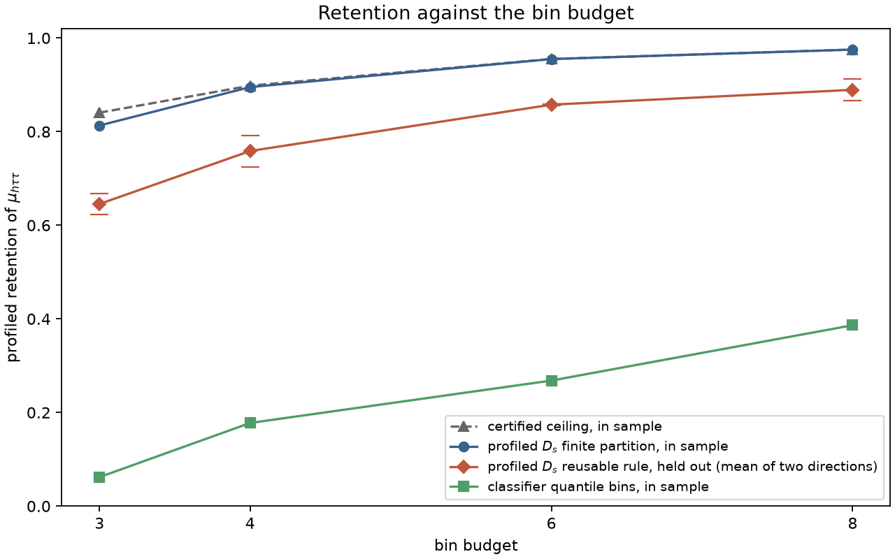
efficient_score_bound supplies the certified ceiling. At six cells, the profiled partition (DExchangeConfig(seed=11), seeded from the bound's own labels) retains 0.9550 against a ceiling of 0.9553: a retention gap of 0.0002, and 0.0003 nats of the profiled log-determinant. It is not merely better than the baselines; it is as good as any six-cell rule of this score space could be, in sample.

Cells	Profiled \(D_s\) partition	Classifier quantile bins	Certified ceiling	Certified gap (nats)
3	0.8131	0.0620	0.8406	0.0332
4	0.8952	0.1776	0.8982	0.0034
6	0.9550	0.2682	0.9553	0.0003
8	0.9753	0.3864	0.9753	0.0000

Held out: every rule built on one half, scored on the other

A partition labels the rows it was optimized on. A search needs a rule, and a rule has to be evaluated on events it never saw. The events are split once (event_split, seed 7), stratified by label, into two halves of 500. Every rule is built on one half and scored on the other, in both directions; the classifier-output rules choose their edges on the reference half. The profiled \(D_s\) rule is fit_quantizer with SoftVoronoiConfig(seed=11, initializer_restarts=8, max_steps=400) and the evaluation half passed as validation=, which is diagnostic only; the held-out number is re-derived from predict_scores and agrees with the library's own validation_profiled_report to every printed digit. The plain-\(D\) rule is the exchange partition of the reference half compiled into its Voronoi rule. Each evaluation half also gets its own certified ceiling, so no held-out number can sit above the best any rule could do on that half.

The parameterization (the physical signal fraction) and both calibration temperatures are the full-sample values, frozen across the split, so both halves' score tables live in one parameterization. The residual coupling -- each half's out-of-fold scores come from fold models that saw some events of the other half -- is second-order and is the standard cross-fitting arrangement.

Rule	Reference half, in sample	Held out, mean of both directions	Held out, direction A→B	Held out, direction B→A	Bootstrap envelope (5th to 95th, both directions)
Profiled \(D_s\) finite partition	0.9673 / 0.9638	--	--	--	--
Profiled \(D_s\) rule	0.9282	0.8576	0.8591	0.8561	0.8051 to 0.9146
Plain \(D\) rule	0.8438	0.8025	0.8191	0.7858	0.7311 to 0.8639
Classifier intervals, max \(S^2/(S+B)\)	0.3294	0.3244	0.2494	0.3994	0.1042 to 0.8063
Classifier logit, equal width	0.4169	0.2712	0.3434	0.1989	0.1088 to 0.8656
Classifier quantile bins	0.2633	0.3682	0.3186	0.4177	0.1206 to 0.8330
Certified ceiling of the evaluation half	--	--	0.9642	0.9699	--

Three numbers of the profiled rule belong together: the finite partition on the reference half (in sample, a labelling of those rows), the reusable rule on the reference half (the cost of being a rule at all: 0.9673 to 0.9282 in one direction), and the reusable rule held out (the cost of new events: to 0.8591). The bootstrap resamples the evaluation events with replacement, 200 times, with the labels travelling with the rows, so it reflects the Monte Carlo sample's size and nothing about how the rule was fitted; the distributions are skewed and bounded by one, which is why percentiles are quoted rather than a standard error. The classifier-output rules' envelopes are wide enough that which of them is best changes from one direction of the split to the other.

Occupancy. The profiled rule's advantage lives in small cells: its smallest evaluation cell holds 2 simulated events in one direction and 15 in the other, while the quantile bins' smallest holds 72. That is the price of resolving the tes direction on a 1,000-event fixture, and it is where the Monte Carlo statistical caveat of the downstream section comes from. Per-cell tables (events, weighted yield, signal share, mean tes score) for every rule and both directions are in cross_evaluation.directions[*].rules[*].evaluation_occupancy of the evidence file.

Held-out budget sweep. The reusable profiled rule, held out, retains 0.6455 at three cells, 0.7586 at four, 0.8576 at six and 0.8893 at eight, against in-sample partitions of 0.8131, 0.8952, 0.9550 and 0.9753 and the ceilings above.

Downstream: the signal-strength fit on the count table

Retention is a property of the score proxy. What a search reports is an uncertainty on \(\mu\) from the count table's own likelihood, and that can be computed from the simulation's actual energy-scale response rather than the classifier's estimate of it. Each reusable rule is applied to every event's copy at all seven committed tes values, giving yield templates \(S_b(\alpha)\) and \(B_b(\alpha)\) per cell, and the Asimov binned-Poisson Fisher matrix at \((\mu,\nu,\alpha)=(1,1,1)\) is \(\sum_b g_b g_b^\top/N_b\) with \(g_b=(S_b, B_b, \partial N_b/\partial\alpha)\). The tes derivative is the slope of a least-squares line through the seven points, because a central difference on a few hundred events is dominated by single events crossing a boundary. The relative expected uncertainty on \(\mu\) is \(\sqrt{[I^{-1}]_{\mu\mu}}\).

The finite partitions cannot enter this table: they label the nominal rows and have no rule to apply to a shifted copy.

Rule, 6 cells, fitted on all events	\(\sigma(\mu)\), tes fixed	\(\sigma(\mu)\), tes floating	with MC statistics, tes floating
Profiled \(D_s\) rule	0.700	0.720	28.6
Plain \(D\) rule	0.735	0.765	30.4
Classifier intervals, max \(S^2/(S+B)\)	0.596	1.909	75.8
Classifier logit, equal width	0.636	1.460	58.0
Classifier quantile bins	0.669	1.190	47.3
Significance cut, 2 cells	0.672	not identified	--
Unbinned proxy score	0.856	0.869	--

With tes fixed every rule measures \(\mu\) about equally well, and the classifier-output rules are slightly ahead: they were built for that question. With tes floating they lose a factor of 1.8 to 3.2, because their counts cannot tell a shifted energy scale from a changed signal strength; the profiled rule loses 3%, the plain-\(D\) rule 4%. This is the scientific content of the study stated in the reported quantity, and it is the reason the walkthrough leads with it.

Three notes on the table:

• The unbinned proxy row is not a floor for the template rows. It is the Fisher information of the classifier-estimated score, \(\sum_i w_i s_i s_i^\top\), divided by the signal fraction; the template rows use the simulation's labels for \(S_b\) and \(B_b\), which the classifier only estimates. The two are on different footings and only the ordering within each footing is meaningful.
• Monte Carlo statistics dominate. The yields are 1,000 rows scaled up by weights near 1580, so the Barlow-Beeston-lite inflation \(\mathrm{Var}(N_b)=N_b+\sum_{i\in b}w_i^2\) is about forty times the Poisson variance. The last column includes it; every absolute number becomes a property of the fixture's Monte Carlo size, and the ranking survives.
• A physical constraint on tes changes nothing here. Adding \(1/0.01^2\) to the tes diagonal moves the profiled rule's \(\sigma(\mu)\) from 0.7198 to 0.7197: the yields self-constrain the energy scale far below a 1% width.

Held out. The same table on each evaluation half, with rules built on the other half:

Rule	A→B, tes fixed	A→B, floating	B→A, tes fixed	B→A, floating
Profiled \(D_s\) rule	0.913	1.145	0.888	0.897
Plain \(D\) rule	0.976	1.026	0.959	0.971
Classifier intervals	0.888	1.405	0.910	1.715
Classifier logit, equal width	0.929	1.447	0.857	1.254
Classifier quantile bins	0.934	1.825	0.922	1.579

On 500 events the count table cannot rank rules whose uncertainties differ by less than about a third: the two ScoreQuant rules trade places between the directions, while every classifier-output rule sits above both in both directions. That is why the all-events table is the one the walkthrough shows, with its in-sample optimism for the rules (the classifier-output rules' edges were chosen on the same labels) stated next to it.

The delta convergence study

delta is the finite-difference half-offset the central-log-ratio classifier is trained at, and it is a numerical differentiation step, not the physical tau-energy-scale uncertainty, which is nearer 1-3%. The score is the derivative of the log density at tes = 1 whatever prior width tes carries downstream, and reading these numbers as a physics uncertainty claim would be wrong.

The headline delta = 0.05 is checked against delta = 0.025 and delta = 0.10, the three points the committed fixture carries; the partitions are in sample, on all events:

\(\delta\)	Minus/plus classifier AUC (weighted)	Near-\(0.5\) fraction	Profiled \(D_s\) retention	Certified ceiling
0.025	0.5379	0.071	0.9552	0.9566
0.05	0.5753	0.065	0.9550	0.9553
0.10	0.6786	0.045	0.9527	0.9532

The minus/plus classifier's own discrimination task grows markedly easier with delta, yet the profiled retention at a fixed six-cell budget barely moves; the correlation between the delta and delta/2 score columns is 0.64, so individual events' estimated scores shift more than the aggregate does. This is the linear-rescaling invariance stated above, seen empirically: the partition built from either column agrees on what matters for this measurement.

What the categories look like

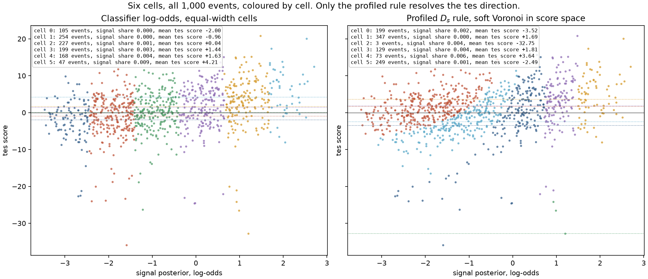
The classifier output is one number, so any binning of it is a set of vertical stripes in this plane. The profiled rule keeps cells whose mean tes score differs, which is what lets the count table register an energy-scale shift as a nuisance change rather than as a signal change.

Discussion

Task: both. optimize_partition for the in-sample partitions and the ceiling, which are statements about this score table; fit_quantizer (and, for plain \(D\), the compile bridge) for the rules, which are the objects a search could deploy and the only ones evaluated held out and downstream. Door: 3, classifier to density ratios to scores, through two different ratio doors -- DensityRatioScore.from_classifier for the rate columns and CentralLogRatioScore for the nuisance-shape column. Criterion / solver: DOptimality and ProfiledDOptimality(interest=("mu_htautau",)) with DExchangeConfig for the finite partitions, SoftVoronoiConfig for the reusable profiled rule, the same pairing nuisance-profiled-ds and michelson-phase use, and for the same reason: finite profiled-\(D_s\) labels have no canonical inductive rule to compile into.

What would change the numbers. A larger fixture. The held-out envelopes and the downstream noise on 500 events are both consequences of 1,000 rows and 665 effective events; the fixture builder needs the network and packages the project does not depend on, so enlarging it is a data decision rather than a code change.

Every number on this page is read from the committed evidence JSON (docs/examples/assets/hep-classifier.json), regenerated deterministically by JAX_ENABLE_X64=1 MPLBACKEND=Agg uv run python -m examples.hep_classifier (about two minutes) and pinned in tests/test_evidence_suite.py. The matching notebook, hep_classifier.ipynb, runs the classifier-to-score bridge live at fast-mode scale and re-derives the same tables.