A Higgs search with a floating energy scale

Simulated collision events are to be reported as a table of 6 counts. The signal strength is the parameter of interest; the tau energy scale is a nuisance that floats in the fit. Which 6 categories keep the most information about the signal strength once the energy scale is free to move?

1. The measurement

A search for the Higgs boson decaying to two tau leptons counts collision events that look like the signal and compares the count with the prediction. The quantity reported is the signal strength $\mu$, the observed signal rate relative to the nominal prediction: $\mu = 1$ means the prediction holds. Two other quantities are estimated at the same time. The background rate $\nu$ scales the events that look like the signal but are not. The tau energy scale $\alpha$ is a calibration parameter: if the detector measures every hadronic tau energy a fraction $\alpha - 1$ too high, every energy-dependent quantity of every event shifts, and the shifted background can imitate a change in $\mu$.

This page is a simulation study on a committed fixture: 1,000 simulated events from the FAIR Universe - HiggsML Uncertainty Challenge Public Dataset, 336 of them signal and 664 background, each carrying a Monte Carlo weight. The weights are far from uniform (a background event stands for roughly five hundred times more collisions than a signal event), so the sample is worth about 665 equally weighted events. The fixture holds row-aligned copies of every event with the energy scale shifted to seven values, which is what makes the effect of $\alpha$ measurable. The energy scale is treated as a free nuisance: nothing on this page constrains it, neither in the choice of categories nor in the numbers reported, and the closing section says what a physical constraint would change.

Nothing here describes how a published measurement is performed. The background processes are merged into one component, the event selection is held fixed under the shift, and the classifiers are ordinary gradient-boosted trees. The choices are recorded on the reference page (opens in a new tab).

2. Why bin the events

The likelihood of a collision event has no closed form: a simulation generates events, and the analysis learns from them. What gets published is a table of counts in a few categories, one expected yield per category per process, and a likelihood built on that table. The categories are the compression. A category boundary that separates signal from background well is not necessarily one that survives a floating energy scale, because the region where signal concentrates is also the region the energy scale moves background through, and a category that cannot tell the two apart hands part of its signal sensitivity to the nuisance.

So the question is not only "which 6 categories separate signal from background" but "which 6 categories keep the signal strength measurable after the background rate and the energy scale have been fitted from the same counts".

3. Three coordinates per event

ScoreQuant does not take events. It takes, for each event, the sensitivity of the event's log likelihood to each parameter: one column for $\mu$, one for $\nu$, one for $\alpha$. Nobody has that likelihood, so the columns are estimated through density ratios. A signal-versus-background classifier, calibrated and divided by its training proportions, gives the two rate columns in closed form. A second classifier trained to tell an event's energy-scale-shifted-down copy from its shifted-up copy gives the energy-scale column as a central difference. Both classifiers are cross-fitted with one fold per event, so no event is scored by a model that saw it or its shifted copies, and both are trained under the Monte Carlo weights, so the ratios they estimate are those of the physical mixture rather than of the simulated event list. That is the whole score construction; its diagnostics, the leakage trap it avoids and the convergence check on the finite-difference step are on the reference page.

import numpy as np

import scorequant as sq
from examples.hep_classifier import SCHEMA, cross_fitted_table, load_fixture

data = load_fixture()
table = cross_fitted_table(data)

assert table.scores.shape == (data.n_events, 3)
assert SCHEMA.parameters == ("mu_htautau", "nu_background", "tes")

Two facts about this score table matter for everything below. It is a proxy: every column came from a trained classifier, so the library records the provenance as an estimated ratio and never describes a result in exact-Fisher language. And the energy-scale column is the noisier of the two constructions: two classifiers trained on disjoint events agree on it only at a correlation of 0.50, and per-event noise in that column biases every retention quoted below downwards.

4. A reusable rule, fitted on half the events

A partition of these 1,000 rows would label these rows and nothing else. A search needs a rule: a function of an event's three coordinates that returns a category, so that a new event, or a shifted copy of an old one, can be categorised. Everything applied below is a rule, and every rule is built on one half of the events and applied to the other.

The events are split once, stratified by label, into two halves of 500. The rule is fitted on the reference half with fit_quantizer, under the profiled criterion: keep the information about mu_htautau that remains after the other two parameters have been profiled out. The evaluation half is passed as a validation sample, which is diagnostic only and never touches the fit.

from examples.hep_classifier.experiment import HEADLINE_BINS, SOLVER_SEED, event_split

halves = event_split(data.is_signal)
reference = table.subset(halves == 0)
evaluation = table.subset(halves == 1)

ds_rule = sq.fit_quantizer(
    reference.sample(),
    validation=evaluation.sample(),
    n_bins=HEADLINE_BINS,
    criterion=sq.ProfiledDOptimality(("mu_htautau",)),
    config=sq.SoftVoronoiConfig(seed=SOLVER_SEED, initializer_restarts=8, max_steps=400),
)
assert ds_rule.information_kind == "supplied_score_surrogate"

Two criteria are compared throughout. Full D-optimality maximises the determinant of the binned information over all three parameters at once: it treats $\mu$, $\nu$ and $\alpha$ as equally worth resolving. Profiled $D_s$ maximises the information about $\mu$ alone after $\nu$ and $\alpha$ have been fitted from the same counts, which is the Schur complement of the binned information. The second is the question this measurement asks. For plain D the finite partition can be compiled into its Voronoi rule; for profiled $D_s$ no such bridge exists, so the reusable rule is fitted directly as a soft Voronoi rule and hardened, exactly as on the Michelson page.

5. What the categories look like

The comparison that matters is with the rule a physicist would build first: slice the signal classifier's output into 6 intervals. The figure draws both rules on the same events, in the plane a physicist can read: the classifier's log-odds against the energy-scale score.

Left: six equal-width cells of the classifier's log-odds. Right: the reusable profiled rule fitted on the same events. Only the right-hand rule resolves the vertical direction, and that direction is the one a floating energy scale moves events along.

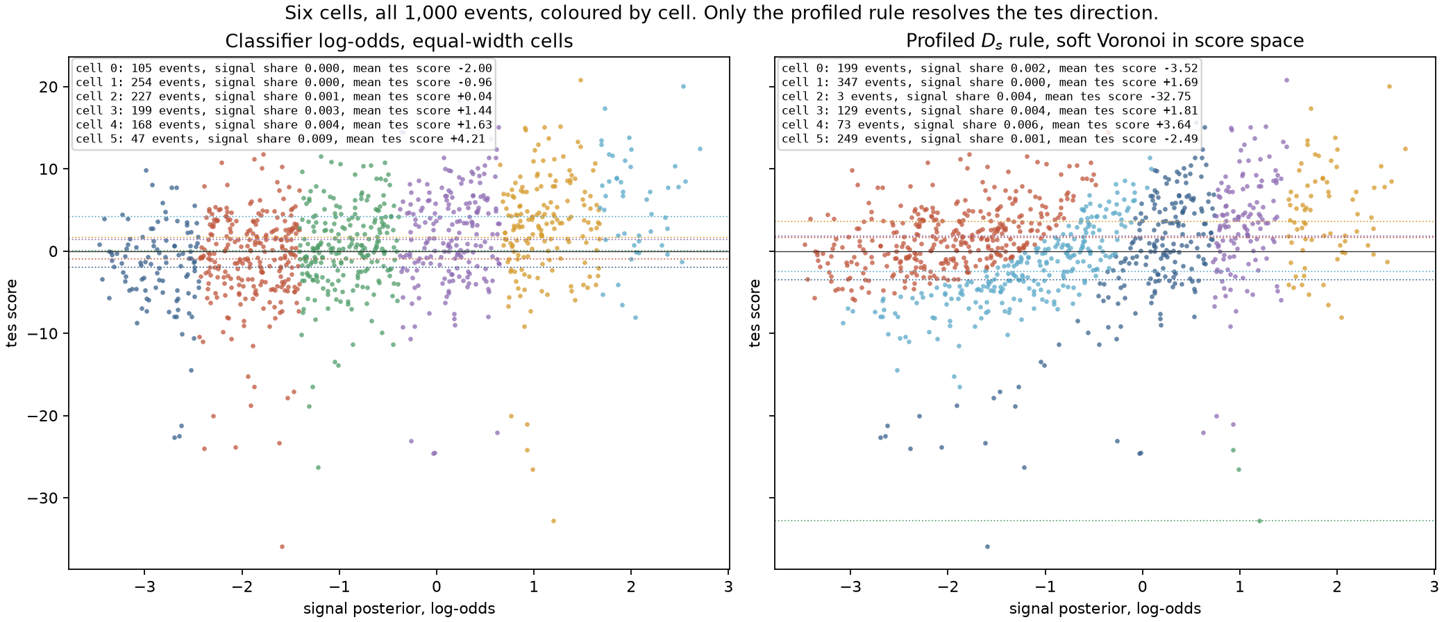
The classifier output is one number, built to separate signal from background. Any binning of it is a set of vertical stripes: it cannot encode a direction it never contained, and the energy-scale direction is precisely that direction. The profiled rule spends its 6 cells differently. It keeps cells whose mean energy-scale score differs, so that when the energy scale moves events between cells the count table registers the movement as a nuisance change rather than as a signal change.

6. Applying the frozen rule

The rule is frozen and applied to the evaluation half, events it has never seen. What a search publishes is the resulting count table: for each category, the expected signal yield and the expected background yield at the nominal energy scale.

labels = ds_rule.predict_scores(evaluation.scores)

signal_yield = np.bincount(
    labels, weights=np.where(evaluation.is_signal, evaluation.weights, 0.0), minlength=HEADLINE_BINS
)
background_yield = np.bincount(
    labels, weights=np.where(~evaluation.is_signal, evaluation.weights, 0.0), minlength=HEADLINE_BINS
)
assert signal_yield.shape == background_yield.shape == (HEADLINE_BINS,)

Applying the same rule to the events' shifted copies gives the yields at every committed energy scale, which is the nuisance template the likelihood needs. Those templates, not the score proxy, are what the next section fits.

7. What the count table can measure

The downstream question is the expected uncertainty on the signal strength from the count table's own Poisson likelihood, with $\nu$ and $\alpha$ floating. It is computed from the yield templates built as above, with the simulation's actual energy-scale response rather than the classifier proxy, as an Asimov expected uncertainty at $\mu = 1$. The table gives it for every rule, once with the energy scale held fixed and once with it floating.

Rule, 6 categories	σ(μ), energy scale fixed	σ(μ), energy scale floating
Profiled $D_s$ rule	0.700	0.720
Plain D rule	0.735	0.765
Classifier intervals, max S²/(S+B)	0.596	1.909
Classifier logit, equal width	0.636	1.460
Classifier quantile bins	0.669	1.190

The uncertainties are relative to the signal strength at this fixture's yields, and the fixture's total weight is a subsample sum rather than the challenge's expected yield, so the absolute values are not a projected sensitivity; the ratios between rows are the result. Read the columns against each other. With the energy scale fixed, every rule does about equally well, and the classifier-output rules are even slightly ahead: they were built for exactly that question. Once the energy scale floats, the classifier-output rules lose between a factor of two and a factor of three, because the counts cannot distinguish a shifted energy scale from a changed signal strength and the fit is forced to trade the two off. The profiled rule loses a few percent. That is the whole scientific lesson of the page, stated in the quantity the measurement reports.

Two caveats belong next to the table. The rules in it were fitted on all 1,000 events (the label-free ScoreQuant rules and the classifier-output rules alike), because on a held-out half the count table is too small to rank rules whose uncertainties differ by less than about a third; the held-out directions, which show the same ordering with that noise, are on the reference page. And the Monte Carlo statistical uncertainty of the yields themselves, which a real analysis would add, is about forty times the modelled Poisson uncertainty here: with it, the profiled rule's σ(μ) becomes 28.6 against 58.0 for the logit bins, and the ranking survives.

8. Retained information, held out

The information view is the same story with a certificate. For each rule the profiled information about $\mu$ that the evaluation half's counts retain is divided by the unbinned profiled information of the same half, both from the score proxy. The chart shows the mean of the two directions of the split.

Profiled information about the signal strength, held out, compared across 5 binning methods

Method	Profiled information about the signal strength, held out
Classifier quantile bins	0.3682
Classifier logit, equal width	0.2712
S²/(S+B) intervals	0.3244
Plain D rule	0.8025
Profiled Ds rule (ScoreQuant)	0.8576
Certified ceiling (reference ceiling)	0.9642

Every rule uses 6 categories, built on one half of the events and scored on the other, averaged over both directions. The dashed line is the certified ceiling of the evaluation halves. Higher is better.

Finite partition on the reference half

0.9673

Exact exchange labels of the reference rows, scored on those rows. In sample, and only a labelling of those rows: it has no predict method.

Reusable rule on the reference half

0.9282

The soft Voronoi rule scored on the rows it was fitted on. The gap to the partition is the price of being a rule at all.

Reusable rule, held out

0.8576

The same rule on the other half. Bootstrap envelope 0.8051 to 0.9146.

Certified ceiling, evaluation half

0.9642

An upper bound on what any rule with this many cells could retain from the evaluation half's own score table, so no held-out number can sit above it.

The profiled rule's three numbers, so that the loss from hardening a partition into a rule is not confused with the loss from applying it to new events. The two directions of the split gave 0.8591 and 0.8561; the bootstrap envelope is the union of both directions' 5th to 95th percentiles over 200 resamplings of the evaluation events.

The classifier-output rules retain a third of the profiled information or less, and their bootstrap envelopes are wide: the best of them, judged on the evaluation half, changes from one direction of the split to the other. The plain D rule keeps 0.8025. The profiled rule keeps 0.8576 with an envelope of 0.8051 to 0.9146, and it does so with cells that are small: its smallest evaluation cell holds 2 simulated events, which is where the Monte Carlo caveat of the downstream section comes from.

On all 1,000 events, in sample, the finite profiled partition retains 0.9550 against a certified ceiling of 0.9553, a gap of 0.0002; the plain D partition retains 0.8238. Those are the numbers a finite-sample study reports, and they are upper references for what a rule can do, not measurements of one.

9. The conventional reference

The most familiar analysis of all, a single threshold on the classifier output chosen to maximise $S/\sqrt{B}$ with a count on either side, is not in the charts above because it does not use the same budget: it has 2 cells. With the energy scale fixed it measures the signal strength about as well as the others, σ(μ) of 0.672. With three parameters floating it measures nothing: two counts cannot determine three quantities, so the profiled information is not a small number but an unidentified model. A cut-and-count analysis needs the energy scale constrained from elsewhere, which is a statement about the analysis, not a defect of the cut.

10. The bin budget

Retained profiled information against the number of cells. The in-sample partition tracks its certified ceiling at every budget; the reusable rule, held out, sits below both and closes on them as the budget grows.

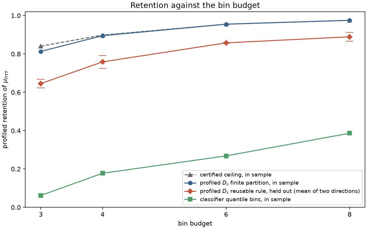
Three cells are the fewest that can identify three parameters, and the held-out rule retains 0.6455 there. At eight cells it retains 0.8893, against 0.9753 for the in-sample partition and a ceiling of 0.9753. The gap between the in-sample and held-out curves is what 1,000 events cost, and it is the reason the page reports both.

11. Limits, and how to reproduce this

The score is a proxy. No unbinned likelihood exists, so every retention on this page is a fraction of the estimated score's information, and the energy-scale column is reproducible only at a correlation of 0.50 between independently trained classifiers. The downstream table above does not depend on the proxy for its energy-scale response, which is why it is the primary result.

The energy scale is unconstrained. Neither the criterion nor any retention number includes an external constraint on $\alpha$. Adding a Gaussian constraint of width 0.01 to the downstream likelihood moves the profiled rule's σ(μ) from 0.720 to 0.720: the yields self-constrain the energy scale far below that width, so a physical constraint changes nothing here.

The fixture is small. 1,000 events, one split, and held-out cells with as few as 2 simulated events. The held-out envelopes are wide for that reason, and the two directions of the split are reported separately rather than only as a mean. A larger fixture is a data decision, not a code change.

Every number on this page is read from the committed evidence file the study writes, regenerated deterministically by

JAX_ENABLE_X64=1 MPLBACKEND=Agg uv run python -m examples.hep_classifier

The classifier construction, the leakage story, the finite-difference convergence check, the per-cell occupancy tables and the held-out downstream directions are on the HEP classifier study (opens in a new tab) page. The theory of the profiled criterion, the efficient score and the certified ceiling is in Nuisance parameters and profiled Ds (opens in a new tab); the two tasks, labelling a fixed table and fitting a rule, are in Two tasks and three optimization levels (opens in a new tab).