Michelson interferometer phase: profiling a fringe-frequency nuisance

This page walks sample partitioning (optimize_partition) and space quantization (fit_quantizer) through Door 2 on an analytic score: a ScoreFunction callback against a bounded IntegrationSource, rather than a precomputed score table or a linear component model. It also runs entirely on the NumPy backend (ExecutionConfig(backend="numpy", ...)), and the model is exact enough that the library's own numbers are a check on the mathematics, not only an illustration of it.

Problem

A Michelson interferometer counts photons along the fringe coordinate. Write the fringe phase \(u=kx\) and record which of \(K\) detector segments each photon lands in. Conditioned on the photon count, the arrival law over \(m\) whole fringes is the fringe shape

\[p(u\mid\varphi,\epsilon)\;\propto\;1+V\cos\!\big((1+\epsilon)u+\varphi\big),\qquad u\in[0,2\pi m),\]

with \(V\) the fringe visibility (fixed, known), \(\varphi\) the phase — the parameter of interest, and \(\epsilon\) a fractional fringe-frequency error — the nuisance. Over a short baseline, a phase offset and a slightly wrong wavenumber are nearly the same signal, which is what makes an unknown \(\epsilon\) the canonical nuisance of interferometric metrology: this is a profiled problem, not a decorative one. Two parameters, one measurement coordinate — the near miss Why bin at all describes in prose, on a model where the answer is exactly computable.

Data

Over whole fringes the normalizer \(Z=\int(1+V\cos(u+\varphi))\,du\) equals the interval length at \(\epsilon_0=0\), so \(\partial_\varphi\log Z=0\) while \(\partial_\epsilon\log Z=V\cos\varphi_0\) does not vanish. At \((\varphi_0,\epsilon_0)=(0,0)\) the conditional score is therefore closed-form:

\[s_\varphi(u)=\frac{-V\sin u}{1+V\cos u},\qquad s_\epsilon(u)=u\,s_\varphi(u)-V.\]

The \(-V\) is the normalizer derivative, not a centering convenience: it is what makes \(E[s_\epsilon]=0\) hold exactly, since \(E[u\,s_\varphi]=V\) independently of the fringe count. Dropping it would leave a score with mean \(+V\) and a wrong information matrix — this is the cleanest available demonstration of the project's "never center scores" invariant, because the origin here is fixed by the model rather than by preference. Both components are bounded because \(1+V\cos u\ge 1-V>0\), so the ScoreFunction finiteness contract holds by construction.

import numpy as np

import scorequant as sq
from examples.michelson_phase import (
    EXECUTION,
    INTEREST,
    N_BINS,
    build_provider,
    build_train_sample,
    closed_form_information,
    equal_width_labels,
    profiled_retention,
    unbinned_profiled_information,
)

provider = build_provider()
sample = build_train_sample(provider, n_nodes=2_000)
assert sample.scores.shape == (2_000, 2)

closed_form = closed_form_information()
information = np.asarray(sq.fisher_information(sample.scores, sample.weights, execution=EXECUTION))
assert abs(float(information[0, 0]) - closed_form["i_phiphi"]) < 1e-12
assert abs(float(information[0, 1]) - closed_form["i_phieps"]) < 1e-12

fringe_density and michelson_score are both 2 pi-periodic in u up to the explicit u * s_phi term in s_epsilon, so deterministic midpoint quadrature of the periodic part converges exponentially rather than at the usual second order. That is what lets fisher_information reproduce \(I_{\varphi\varphi}=1-\sqrt{1-V^2}\) and \(I_{\varphi\epsilon}=I_{\varphi\varphi}\,u_{\max}/2\) to machine precision at only a few thousand nodes — the closed forms are a check on the library, not merely a description of it. \(I_{\epsilon\epsilon}\) has no comparably tidy form; the full study pins it numerically at 41.5392. Together the three give a correlation of \(+0.872\) between \(s_\varphi\) and \(s_\epsilon\) — strong enough that profiling the phase against the frequency costs 76.0% of the phase information before any binning at all: \(0.2\to 0.047938\).

API walkthrough

The profiled ceiling, and why every number below is measured against it

unbinned_profiled_information Schur-completes the nuisance column out of fisher_information directly, no partition required. This is the ceiling every phase-retention number in this page is stated against — never \(I_{\varphi\varphi}\), which is not available to an analyst who does not know \(\epsilon\).

reference = unbinned_profiled_information(sample.scores, sample.weights)
cost_of_profiling = 1.0 - reference / closed_form["i_phiphi"]
assert 0.75 < cost_of_profiling < 0.77

Three partitions of the same score table

optimize_partition runs on provider.score(X), so the observation-to-score step stays visible for all three labelings: naive equal-width detector segments, DOptimality, and ProfiledDOptimality seeded from the certified efficient-score bound.

n_bins = N_BINS
equal_labels = equal_width_labels(sample.observations, n_bins)

d_partition = sq.optimize_partition(
    sample.scores,
    weights=sample.weights,
    n_bins=n_bins,
    criterion=sq.DOptimality(),
    config=sq.DExchangeConfig(seed=4),
    execution=EXECUTION,
)
bound = sq.efficient_score_bound(
    sample.scores, interest=INTEREST, weights=sample.weights, n_bins=n_bins, execution=EXECUTION
)
profiled_partition = sq.optimize_partition(
    sample.scores,
    weights=sample.weights,
    n_bins=n_bins,
    criterion=sq.ProfiledDOptimality(interest=INTEREST),
    config=sq.DExchangeConfig(seed=4),
    initial_labels=bound.labels,
    execution=EXECUTION,
)

equal_retention = profiled_retention(sample, equal_labels, n_bins)
d_retention = profiled_retention(sample, np.asarray(d_partition.labels), n_bins)
ds_retention = profiled_retention(sample, np.asarray(profiled_partition.labels), n_bins)

assert equal_retention < d_retention < ds_retention
assert bound.gap_to(profiled_partition) < 1e-3

ProfiledDOptimality stays within a certified fraction of a percent of the efficient-score ceiling; DOptimality — the wrong criterion for this question — leaves visibly more on the table, even though it is optimal for the whole two-parameter matrix.

Equal-width segments alias against the fringe period

Four equal segments over four whole fringes make each segment exactly one period, so by periodicity every segment's mean score is identical, the between-cell matrix is rank-deficient, and the naive rule retains exactly nothing of the phase.

labels_four = equal_width_labels(sample.observations, 4)
retention_four = profiled_retention(sample, labels_four, 4)
assert retention_four < 1e-9

This is aliasing between the segmentation and the fringe period, and it is a real hazard: the full study also shows a naive rule getting worse going from eight bins to ten, because ten segments over four fringes is 2.5 per fringe and aliases again. Refining a partition can only help — but only when it genuinely refines, and an equal-width rule at a new bin count is not a refinement of the old one.

The compile bridge, and the profiled refusal

The DOptimality partition is exchange-stable, so compile_quantizer() succeeds. The profiled partition has no canonical inductive rule to compile into, and refuses instead.

assert d_partition.exchange_stable is True
compiled = d_partition.compile_quantizer(execution=EXECUTION)

try:
    profiled_partition.compile_quantizer(execution=EXECUTION)
    raise AssertionError("a profiled-D partition must refuse compile_quantizer()")
except sq.RefusalError as error:
    refusal_message = str(error)

assert refusal_message.endswith("[CE-DS-GLOBAL-GEOMETRY-001]")

The reusable rule on the missing route

fit_quantizer(source, provider=provider, ...) with source the same bounded IntegrationSource — the input route this page exists to cover. An exchange-stable DOptimality partition compiles into a Mahalanobis rule automatically, so hardening_gap is exactly zero; ProfiledDOptimality has no such bridge, so a reusable profiled rule must be fitted as one, which SoftVoronoiConfig does.

from examples.michelson_phase import build_integration_source, reusable_rules

source = build_integration_source()
fitted = reusable_rules(provider, source, sample, n_bins=n_bins, soft_steps=80)
rules = {row.key: row for row in fitted.rows}

assert rules["d_rule"].hardening_gap == 0.0
assert abs(rules["ds_rule"].hardening_gap) < 1e-2  # soft and hard nearly agree either way

# Both rows report the same quantity against the same ceiling, so they compare.
assert rules["ds_rule"].profiled_retention > rules["d_rule"].profiled_retention
# A nearest-centre rule is a restricted family; the finite partition retains more.
assert rules["ds_rule"].profiled_retention < ds_retention

Read the two columns separately. criterion_efficiency is what each rule scores on the criterion it optimized, and the two are not comparable: the plain rule's number is an overall D-efficiency and the profiled rule's is a profiled retention, on different denominators. The column that does compare is profiled_retention, which puts both rules' own labels through the same profiled ceiling as the sweep above — and there the profiled rule wins, which is the whole reason it exists. A rule can score well on its own criterion and still be the wrong rule for the question being asked.

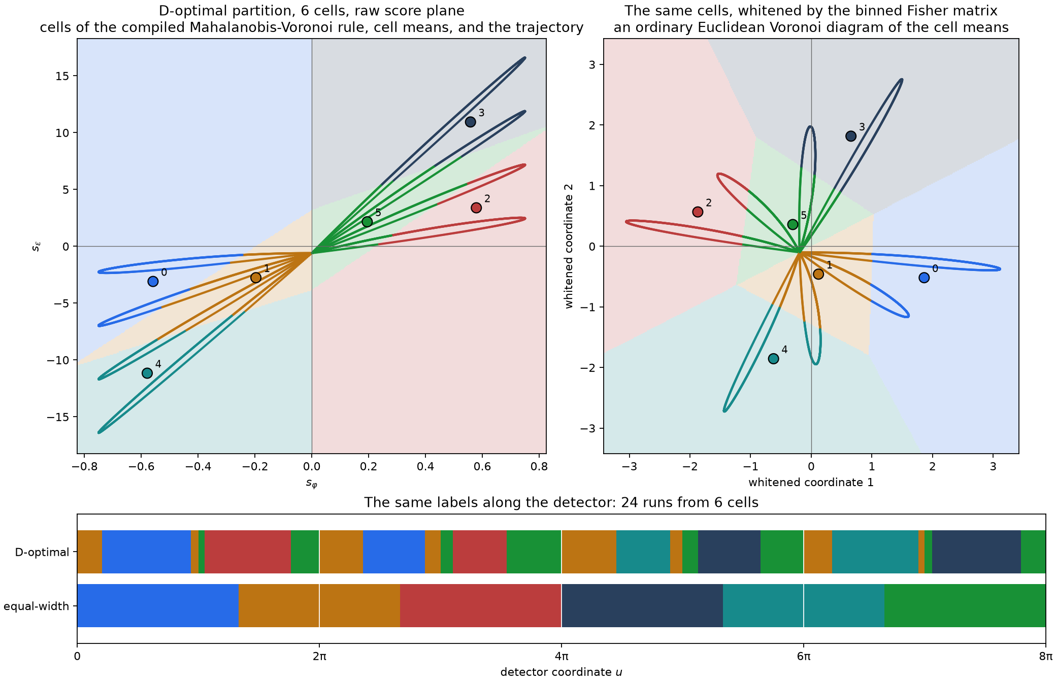
The comb, and the fragments

The score depends on u only through the fringe phase, so a connected score-space cell pulls back to one interval per fringe: the compiled six-cell rule is a comb of twenty-four detector runs, not six. run_diagnostics counts the runs with the two detector ends joined, since s(0) and s(u_max) are the same score vector.

from examples.michelson_phase import run_diagnostics

d_geometry = run_diagnostics(sample, np.asarray(d_partition.labels), n_bins=n_bins)
# Two cells at the origin are crossed twice per loop; the four outer cells
# each own the tips of a pair of loops.
assert sorted(d_geometry.runs_per_bin) == [2, 2, 2, 2, 8, 8]

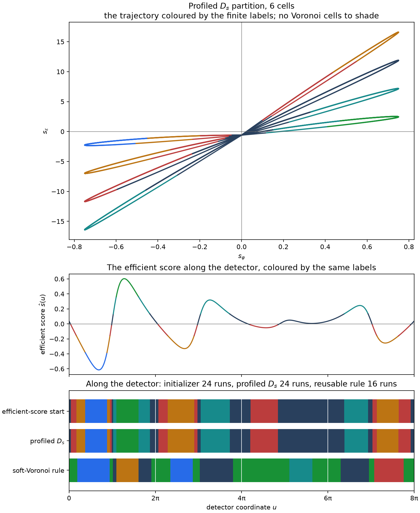
The profiled partition combs the detector too, and adds something the D partition does not: a handful of very narrow runs where the efficient score crosses zero steeply. profiled_trace shows where they come from -- the certified interval initializer already has them, and the exchange that follows changes few labels and gains little -- and smoothing_ladder shows what they are worth, by absorbing every run narrower than a threshold into its wider neighbour and re-measuring the profiled retention.

from examples.michelson_phase import profiled_trace, smoothing_ladder, sweep_bin_budget

reference = unbinned_profiled_information(sample.scores, sample.weights)
headline = sweep_bin_budget(sample, reference, budgets=(n_bins,))[0]
trace = profiled_trace(sample, headline)
assert trace.exchange_stable
assert trace.initial.narrow_runs >= trace.final.narrow_runs
assert 0.0 <= trace.retention_gain < 1e-2

ladder = smoothing_ladder(sample, headline.profiled_labels, n_bins=n_bins)
assert all(row.retention <= trace.final_retention + 1e-12 for row in ladder)

Analysis

The full study runs 8,000 deterministic midpoint-quadrature nodes (2,000 under SCOREQUANT_EXAMPLE_FAST) and sweeps the bin budget. Every retention below is profiled phase information against the unbinned profiled ceiling (0.047938), never against \(I_{\varphi\varphi}\):

\(K\)	equal-width segments	D-optimal	profiled-\(D_s\)-optimal	bound gap
4	0.0000	0.7227	0.8629	5.0e-03
6	0.2054	0.7995	0.9483	2.5e-05
8	0.7247	0.8806	0.9714	6.5e-05
10	0.5653	0.9267	0.9817	1.2e-04

Three things in that table are the page's reason to exist. Equal-width segments retain exactly nothing at \(K=4\), for the periodicity reason above. Adding segments can make the naive rule worse — 0.7247 at eight bins down to 0.5653 at ten — because ten segments over four fringes is 2.5 per fringe and aliases again, while eight is a clean two per fringe. And DOptimality is provably not the phase criterion: at every swept budget it returns different labels from ProfiledDOptimality and retains visibly less phase information, while the profiled solver's gap to the certified efficient-score ceiling never exceeds 5.0e-03 — provably close to the best any \(K\)-cell rule of the whole score space can do.

No downstream likelihood fit lives here; nuisance-profiled-ds already carries that arc, and the value of this page is the exactness of the model, not a second Poisson fit. No ScalarDPConfig run either: the score space is rank 2, so the interval dynamic program does not apply, and saying so plainly is more useful than demonstrating a refusal nobody asked about.

Discussion

Task: both — sample partitioning for the headline sweep and the compile bridge, then space quantization for the reusable rule on the missing route. Door: 2, an analytic ScoreFunction against a bounded IntegrationSource — the one input route with no example before this page. Criterion / solver: DOptimality with exact exchange for the compiled route; ProfiledDOptimality with exact exchange (seeded from efficient_score_bound) for the finite partition and with SoftVoronoiConfig for the reusable rule, since finite profiled-D labels have no compile bridge.

Everything on this page runs on ExecutionConfig(backend="numpy", precision="float64", device="cpu") — the portable CPU runtime that runs the same shared mathematics as the JAX default, demonstrated here end to end rather than only unit-tested.

The generator, examples/michelson_phase.py, runs the full 8,000-node sweep, the diagnostics and both figures. The matching notebook, michelson_phase.ipynb, reproduces the study cell by cell, and the portal walkthrough retells it as a two-act article.