Bin by score, not by feature

Binning loses information in exactly one way: by putting events with different scores in the same bin. So the bins belong in score space.

Counting in bins

Many measurements end in a histogram. Events are sorted into a few bins, the counts are recorded, and a parameter $\theta$ is fitted to the counts. The bins are usually drawn in the space the events were measured in: equal slices of an energy, a position on a detector, the output of a classifier.

That compression has a cost, and Fisher information measures it. Its inverse is the smallest variance an unbiased estimate of $\theta$ can reach, so bins that keep half of the information double that bound.

What a bin forgets

The score of an event is the derivative of its log density with respect to the parameter, $s(x)=\partial_\theta\log p(x\mid\theta)$, at a reference value $\theta_0$. It says how strongly, and in which direction, the probability of that event responds to a change of $\theta$. Give event $i$ the probability $w_i$ and score $s_i$. The information of the unbinned data is the weighted second moment of the score, $I=\sum_i w_i\,s_is_i^\top$; with several parameters the score is a vector and $I$ a matrix.

A bin $b$ holds probability $W_b$, and its count responds to $\theta$ through the mean score $\mu_b$ of the events it holds. The counts therefore carry $I_{\rm bin}=\sum_b W_b\,\mu_b\mu_b^\top$, and the difference is

$$I-I_{\rm bin} = \sum_b\sum_{i\in b} w_i\,(s_i-\mu_b)(s_i-\mu_b)^\top .$$

This is the familiar split of a second moment into a between-group and a within-group part. The information lost is exactly the scatter of the score inside each bin. Nothing else enters: not how far apart the events were in the measured space, not whether a bin is one piece, not how wide it is.

The reason this points to score space is simple: two events with the same score are interchangeable for the measurement, however far apart they were recorded, while two neighbours with scores of opposite sign cancel when they share a bin. Good bins collect events with similar scores.

A fringe pattern

An interferometer makes the point sharply. Photons land on a detector in a fringe pattern, $p(u\mid\varphi)\propto 1+V\cos(u+\varphi)$, and the phase $\varphi$ is the only parameter. Its score at $\varphi=0$ is

$$s(u)=-\frac{V\sin u}{1+V\cos u},$$

positive on one slope of each fringe, negative on the other, and zero at the bright and dark extremes.

Cut a detector spanning 4 fringes into 4 equal segments, one per fringe. A phase shift slides the pattern sideways, but every segment still holds exactly one full period, so no count changes. Each segment's mean score is zero, all the information sits in the scatter inside the segments, and the counts keep 0.00 of it.

Now cut the score instead, into the 4 intervals of $s$ that keep the most information. Each interval collects pieces of every fringe, so along the detector it is a comb of strips. The same number of counts now keeps 0.94 of the information.

Left: the phase score along the detector, coloured by the four score intervals; the dashed lines mark the four equal segments. Right: the fraction of the phase information kept by equal segments and by score intervals, as the number of bins grows.

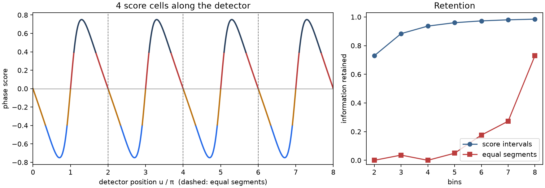
Equal segments are not always this bad. At other budgets they keep part of the information, but how much depends on how the segments happen to line up with the fringes, and more segments are not always better. The score intervals keep more at every budget shown.

One caveat belongs here. The score is evaluated at a reference value of the parameter, so bins drawn from it are best for parameters near that value; far from it, bins drawn at another reference value could keep more.

Several parameters

With several parameters the identity is the same, and so is its conclusion: the cells belong in score space. The cells are then regions of a plane or of a higher-dimensional space, and choosing them means deciding what to trade between parameters. The next post is about that choice. The interferometer walkthrough carries the fringe example further, with the fringe frequency unknown as well.

In code

ScoreQuant takes a weighted table of scores and returns the bins. For one parameter the best intervals of the score are found exactly:

import numpy as np

import scorequant as sq

VISIBILITY = 0.6
N_BINS = 4

u = np.linspace(0.0, 8.0 * np.pi, 8_000, endpoint=False) + np.pi / 8_000
weights = 1.0 + VISIBILITY * np.cos(u)  # photon density, up to a constant
scores = (-VISIBILITY * np.sin(u) / weights)[:, None]

segments = (u // (2.0 * np.pi)).astype(int)  # one equal segment per fringe
by_position = sq.information_report(scores, segments, weights, n_bins=N_BINS)

rule = sq.fit_quantizer(
    sq.ScoreSample(scores, weights),
    n_bins=N_BINS,
    criterion=sq.DOptimality(),
    config=sq.ScalarDPConfig(),
)
by_score = sq.information_report(scores, rule.predict_scores(scores), weights, n_bins=N_BINS)

by_position.geometric_mean_retention is zero up to rounding, and by_score.geometric_mean_retention is the value above. The fitted rule assigns a bin to any new score. When the density cannot be written down, the score can still come from a classifier, as the density-ratio walkthrough shows.