From a classifier to Fisher-preserving bins

When component densities are unavailable but labelled simulations are, a calibrated classifier can provide the density ratios needed to construct a score. ScoreQuant can then compress that estimated score into a small number of bins — but the information it reports is only as reliable as the score it was given.

The two lanes of this page. Along the top, the workflow a real analysis can run: labelled simulations train a classifier, its calibrated posteriors become a density ratio and then a score, and ScoreQuant compresses that score into hard bins. Along the bottom, the check only a synthetic model allows: the exact densities give the exact score, and the same fitted bins are evaluated against it.

1. A mixture fit without an explicit likelihood

Consider a familiar inference problem. Each observed event comes from one of two components — signal or background — and the quantity we want to measure is the signal fraction $\theta$.

If the component densities were known, the event density would be

$$p(x\mid\theta) = \theta\,\phi_{\rm sig}(x) + (1-\theta)\,\phi_{\rm bkg}(x).$$

In many realistic analyses, however, $\phi_{\rm sig}(x)$ and $\phi_{\rm bkg}(x)$ cannot be evaluated. The observation $x$ may be high-dimensional, and the components may be defined only through simulation. What we do have are labelled simulated events from each component — exactly the setting in which a classifier is easy to train.

This walkthrough uses a deliberately simple synthetic mixture so that we can see both sides of the problem. Signal events follow

$$\phi_{\rm sig}=\mathcal N(1.0,\,0.5^2),$$

background events follow

$$\phi_{\rm bkg}=\mathcal N(0.0,\,1.5^2),$$

and the reference point $\theta_0$ is fixed at a signal fraction of 0.30.

For the algorithm, we will pretend that the two densities are unavailable and use only labelled samples and a classifier. Because this is a controlled example, we can also evaluate the exact densities afterward and ask a question that a real analysis usually cannot answer directly:

when ScoreQuant says that a set of bins retains almost all available information, how much of that statement comes from the binning — and how much depends on the classifier that supplied the score?

That distinction is the point of this walkthrough. The program that produces every number below is examples/door3_classifier.py; its full per-rung table is on the reference page Door 3, classifier-estimated density ratios (opens in a new tab).

2. From classifier probabilities to a score

Suppose the classifier was trained on signal and background samples mixed in known proportions $\pi_{\rm sig}$ and $\pi_{\rm bkg}$. If

$$\eta_{\rm sig}(x)=P_{\rm train}(\mathrm{sig}\mid x), \qquad \eta_{\rm bkg}(x)=1-\eta_{\rm sig}(x),$$

then Bayes' rule gives

$$r(x) = \frac{\phi_{\rm sig}(x)} {\phi_{\rm bkg}(x)} = \frac{\eta_{\rm sig}(x)/\pi_{\rm sig}} {\eta_{\rm bkg}(x)/\pi_{\rm bkg}}.$$

So a classifier gives the required density ratio only if its probabilities are calibrated and the training class proportions are known.

For the mixture

$$p(x\mid\theta) = \theta\,\phi_{\rm sig}(x) + (1-\theta)\,\phi_{\rm bkg}(x),$$

the score is, by definition,

$$s(x;\theta) = \frac{\partial}{\partial\theta} \log p(x\mid\theta) = \frac{ \phi_{\rm sig}(x)-\phi_{\rm bkg}(x) }{ \theta\,\phi_{\rm sig}(x) + (1-\theta)\,\phi_{\rm bkg}(x) }.$$

Dividing numerator and denominator by $\phi_{\rm bkg}(x)$ gives

$$s(x;\theta) = \frac{r(x)-1} {\theta r(x)+(1-\theta)}.$$

At the reference point $\theta_0$, this is the score passed to ScoreQuant.

The important point is that the score is defined from the likelihood, but evaluating it does not require the two component densities separately. Their ratio is sufficient.

In our synthetic example the exact Gaussian densities are also known, so we can compute the exact score afterward and use it as an oracle for validation.

3. A controlled experiment

We use the known Gaussian model only to generate a controlled test. The quantizer is fitted on 400 events drawn from the reference mixture at $\theta_0$ equal to 0.30, and another 600 events are kept aside for evaluation.

import numpy as np
from sklearn.linear_model import LogisticRegression

import scorequant as sq


signal_mu, signal_sigma = 1.0, 0.5
background_mu, background_sigma = 0.0, 1.5
reference_fractions = (0.3, 0.7)


def draw(seed, n, signal_fraction):
    rng = np.random.default_rng(seed)
    is_signal = rng.random(n) < signal_fraction

    x = np.where(
        is_signal,
        rng.normal(signal_mu, signal_sigma, n),
        rng.normal(background_mu, background_sigma, n),
    )
    return x[:, None]


train_observations = draw(2026, 400, reference_fractions[0])
test_observations = draw(999, 600, reference_fractions[0])

The classifier is trained separately on balanced signal and background samples. We repeat the experiment with 15, 60 and 300 labelled events per component.

Because the exact log-density ratio of two Gaussians is quadratic in $x$, we use logistic regression with the features $x$ and $x^2$. The model class is therefore expressive enough for this example; the experimental control we vary is the amount of labelled training data.

Everything downstream stays fixed: the reference mixture, the quantizer training sample, the held-out sample, the budget of 4 bins, and the ScoreQuant optimization.

4. Fit the bins

Training the classifier remains application code. ScoreQuant enters once the classifier can provide calibrated posterior probabilities.

We first define the quadratic feature map and the classifier training step:

def make_features(x):
    return np.column_stack([x, x**2])


def train_classifier(seed, n_per_class):
    rng = np.random.default_rng(seed)

    x_signal = rng.normal(signal_mu, signal_sigma, n_per_class)
    x_background = rng.normal(background_mu, background_sigma, n_per_class)

    x = np.concatenate([x_signal, x_background])
    y = np.concatenate([
        np.zeros(n_per_class),
        np.ones(n_per_class),
    ])

    return LogisticRegression(max_iter=1000).fit(make_features(x), y)

The classifier output is then wrapped as a density-ratio score provider:

def classifier_provider(model, description):
    def predict(x):
        values = np.asarray(x)[:, 0]
        return model.predict_proba(make_features(values))

    return sq.DensityRatioScore.from_classifier(
        predict,
        [0.5, 0.5],
        sq.MixtureParameterization(list(reference_fractions)),
        description=description,
    )

For the smallest training sample:

estimated = classifier_provider(
    train_classifier(seed=101, n_per_class=15),
    "logistic regression, 15 events per class",
)

quantizer = sq.fit_quantizer(
    sq.ObservationSample(train_observations),
    provider=estimated,
    n_bins=4,
    criterion=sq.DOptimality(),
    config=sq.DExchangeConfig(seed=7),
)
assert quantizer.information_kind == "supplied_score_surrogate"

The provider performs the conversion derived above: classifier posteriors $\rightarrow$ density ratio $\rightarrow$ estimated score $\hat s(x;\theta_0)$. From that point on, fit_quantizer treats it like any other score source and finds 4 hard bins that preserve as much information in that score as possible.

The result is labelled supplied_score_surrogate, not exact_fisher, and that label is derived from the declared provenance rather than chosen. However good the classifier is, a classifier-backed result never claims exact Fisher semantics.

We repeat the same procedure for classifiers trained with 60 and 300 events per component. The quantizer is unchanged; only the score supplied to it changes.

5. Reported versus achieved information

There are two different questions we can ask about the fitted bins.

First, how much information do they preserve in the estimated score supplied to ScoreQuant? This is the quantity the library can report in a real analysis.

estimated_test_scores = estimated.score(test_observations)

reported = float(
    quantizer.evaluate_scores(
        estimated_test_scores
    ).geometric_mean_retention
)

In our controlled example we can ask a second question. Because the Gaussian component densities are known, we can compute the exact score directly:

def normal_density(x, mu, sigma):
    return np.exp(-0.5 * ((x - mu) / sigma) ** 2) / sigma


def exact_score(x):
    values = np.asarray(x)[:, 0]

    signal = normal_density(values, signal_mu, signal_sigma)
    background = normal_density(values, background_mu, background_sigma)

    theta = reference_fractions[0]

    score = (
        (signal - background)
        / (theta * signal + (1.0 - theta) * background)
    )

    return score[:, None]

We keep the fitted bins unchanged, assign the held-out events using the estimated score, and then evaluate those same labels against the exact score:

labels = np.asarray(
    quantizer.predict_scores(estimated_test_scores)
)

achieved = float(
    sq.information_report(
        exact_score(test_observations),
        labels,
        n_bins=quantizer.n_bins,
    ).geometric_mean_retention
)

The distinction is important:

• reported retention measures what the bins preserve about $\hat s(x;\theta_0)$;
• achieved retention measures what the same bins preserve about the exact $s(x;\theta_0)$.

Repeating the experiment for the three classifier training sizes gives:

Events per component	Reported	Achieved
15	0.9658	0.8847
60	0.9691	0.9521
300	0.9700	0.9665

The surrogate caveat, drawn. The left bar of each pair is what the library can honestly say about the vectors it was handed; the right bar is what those labels were worth. They converge only as the classifier does.

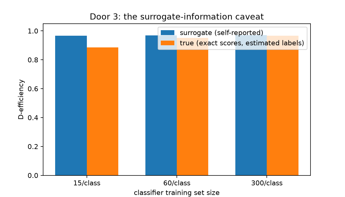
The reported retention barely changes: ScoreQuant is consistently good at preserving the score it receives. The achieved retention tells a different story. With only 15 events per component, the bins reach a D-efficiency of 0.9658 against the classifier-derived score but only 0.8847 against the exact one — a gap of 0.0811 that the self-report cannot see. As the classifier improves the two numbers converge, and by 300 events per component the gap is down to 0.0035.

This is the central limitation of a surrogate score. ScoreQuant can measure the information lost by quantization, but it cannot recover or measure information that was already lost when the score was estimated.

6. A simple closure check

In a real analysis we do not know the exact score, so we cannot repeat the reported-versus-achieved comparison above. We can still perform a simple consistency check on the classifier probabilities themselves.

Our classifiers are trained on balanced samples: half signal and half background. For a large independent sample drawn from that same balanced mixture, a calibrated classifier should therefore predict, on average,

$$\langle P(\mathrm{sig}\mid x)\rangle \approx 0.5, \qquad \langle P(\mathrm{bkg}\mid x)\rangle \approx 0.5.$$

ScoreQuant converts these probabilities into component density ratios by dividing by the corresponding training fractions. With balanced training,

$$\rho_{\rm sig}(x) = \frac{P(\mathrm{sig}\mid x)}{0.5}, \qquad \rho_{\rm bkg}(x) = \frac{P(\mathrm{bkg}\mid x)}{0.5}.$$

Their averages should therefore be close to one.

We test this on a large independent sample of 50,000 events drawn from the same balanced mixture:

closure_observations = draw(4242, 50_000, 0.5)

closure = sq.ratio_closure_report(
    estimated.ratio(closure_observations),
    np.ones(len(closure_observations)),
)

Repeating the check for the three classifier training sizes gives:

Events per component	Closure residual
15	0.0420
60	0.0185
300	0.0032

The residual decreases as the classifier improves. This is useful because, unlike the achieved-information test above, it does not require knowing the exact score.

The check must, however, use the same mixture in which the classifier probabilities were defined. Our classifier was trained with equal signal and background fractions, so the closure sample must be balanced too.

If we instead evaluate the same check on the reference mixture, whose signal fraction is 0.30, the residual rises to 0.1800 even for an exactly correct ratio — larger than the worst of the three above. Nothing is wrong with the ratio; we have simply averaged it over the wrong distribution.

Closure is therefore a useful diagnostic, but not a proof of correctness. A large residual exposes an inconsistency; a small residual only shows that this normalization check is satisfied.

7. Do optimized bins matter here?

This example has only one score coordinate and 4 bins. In such a simple setting, we should not expect a sophisticated partition to outperform ordinary one-dimensional binning by much.

To check that, we compare the ScoreQuant partition with quantile and equal-width bins built from the same estimated score.

Classifier training	Quantile bins	Equal-width bins	ScoreQuant
15 events per component	0.8842	0.8648	0.8847
300 events per component	0.9378	0.9678	0.9665

All numbers are evaluated on the held-out sample against the exact score. A value of one would mean that the bins retain all Fisher information available in that score.

The differences are small. Fitting the partition wins by at most 0.0155, at 60 events per component. With the best-trained classifier, equal-width binning even slightly outperforms the fitted partition: 0.9678 against 0.9665. A quantizer fitted directly from the exact score reaches 0.9724 at the same bin budget.

That is a useful boundary case rather than a failure of the example. With one smooth score coordinate, choosing the bin boundaries is not the difficult part of the problem. The important question on this page is instead whether the score supplied to the quantizer is trustworthy.

The advantage of ScoreQuant becomes more consequential when several score coordinates must be compressed simultaneously, or when an apparently natural one-dimensional binning aliases the information. Those cases are covered by the other walkthroughs.

8. Takeaway

A classifier can make ScoreQuant usable even when the event-level likelihood cannot be evaluated directly. For the mixture considered here, calibrated classifier probabilities determine the component density ratio, and that ratio is sufficient to reconstruct the score at the reference point.

The important limitation is equally clear: ScoreQuant can optimize and measure the information retained from the score it receives, but it cannot recover information that was already lost when that score was estimated.

In this controlled example we could see both effects separately because the exact Gaussian model was known. In a real analysis that oracle is usually unavailable, so classifier calibration and ratio diagnostics become part of the inference pipeline rather than optional preprocessing.

The binning problem itself was deliberately simple: one score coordinate and 4 bins. That made it possible to isolate the classifier-to-score step without introducing the genuinely multivariate geometry for which ScoreQuant is designed. Other walkthroughs address that harder regime.