Phase Estimation in a Michelson Interferometer

A continuous measurement with an analytically known score is to be reported through a fixed number of bins $K$. One parameter is of interest and the others are nuisances. The bins should preserve as much Fisher information as possible.

1. The Michelson interferometer

A Michelson interferometer splits a coherent beam of light into two perpendicular arms. Each beam is reflected by a mirror, returns to the beam splitter, and the two beams are recombined on a detector. Their relative phase is set by the difference in optical path length between the arms.

Schematic optical layout. The segmented detector shows the equal-width baseline.

The beams have a finite transverse width, so they overlap over an area rather than at a point. If the two wavefronts are slightly tilted with respect to each other, the relative phase varies with position across the detector, and the intensity alternates between bright and dark bands. These are interference fringes, or simply fringes.

For a nearly linear phase variation along one detector coordinate $u$,

$$I(u)\propto 1+V\cos(ku+\varphi),$$

where $V$ is the fringe visibility (the contrast of the pattern), $k$ is the spatial fringe frequency, and $\varphi$ is the phase offset. A change in the optical path difference shifts $\varphi$ and moves the whole pattern across the detector. The tilt is only what produces spatial fringes; it is not a parameter of the statistical model below.

Albert A. Michelson introduced the instrument in the late nineteenth century. Gravitational-wave detectors such as LIGO use the same interference principle with far more elaborate optics.

2. Why bin the measurement?

A real interferometric detector is not the ideal model above. Illumination, detector efficiency, fringe visibility, background, optical aberrations and calibration errors all vary with position. Describing them at full detector resolution can require a large nuisance model that is hard to validate.

Binning replaces point-by-point response modelling with the integrated response of a small number of regions. The nuisance model then has a few calibrated quantities instead of one per pixel.

Once the measurement is described by $K$ bins, the bins still have to be defined. Different partitions preserve different amounts of information.

3. Measurement model

The detector is described by a dimensionless coordinate $u$, scaled so that one fringe period has length $2\pi$. The detector spans 4 fringes, so

$$u\in[0,8\pi).$$

The position of one detected photon has density

$$p(u\mid\varphi,\epsilon) \propto 1+V\cos\!\bigl((1+\epsilon)u+\varphi\bigr).$$

Here $\varphi$ is the phase, ultimately the parameter of interest. The visibility is fixed at $V={}$0.60. The parameter $\epsilon$ is a small fractional error in the spatial fringe frequency: it changes the fringe spacing across the detector, so an unknown $\epsilon$ can partly imitate a phase shift.

All scores and information matrices are evaluated at the reference point

$$(\varphi_0,\epsilon_0)=(0,0).$$

Photon density along the detector at visibility 0.60, over 4 fringe periods. The 6 equal-width bins are the baseline readout.

4. The analytic score

ScoreQuant works with the score of each observation, the gradient of the log density with respect to the parameters. Here it is known in closed form. At the reference point,

$$s_\varphi(u) = -\frac{V\sin u}{1+V\cos u}, \qquad s_\epsilon(u) = u\,s_\varphi(u)-V.$$

The phase score is largest in magnitude on the slopes of a fringe, where a small phase shift changes the intensity most, and vanishes at the bright and dark extrema. The frequency score is the same local sensitivity multiplied by $u$, because a frequency error accumulates across the detector. Its constant term $-V$ is the derivative of the normalization of the density with respect to $\epsilon$; without it the score would not have zero mean and the Fisher matrix would be wrong.

Phase score $s_\varphi(u)$ along the detector.

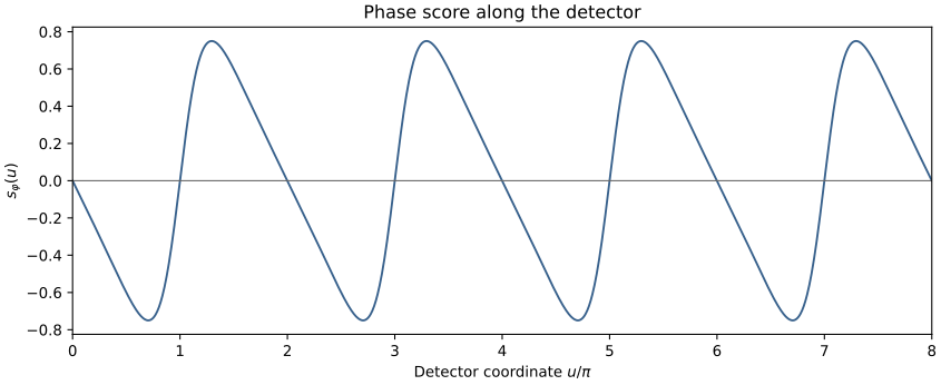
The score is supplied to ScoreQuant as a function of the observation. Fixed model constants are uppercase; computed arrays are lowercase.

import numpy as np
import scorequant as sq

EXECUTION = sq.ExecutionConfig(backend="numpy", precision="float64", device="cpu")

VISIBILITY = 0.60
N_FRINGES = 4
U_MAX = 2.0 * np.pi * N_FRINGES

SCHEMA = sq.ScoreSchema(("phase", "fringe_frequency"))
INTEREST = SCHEMA.select("phase")


def fringe_density(observations):
    """Normalized photon density along the detector at the reference point."""
    u = np.asarray(observations)[:, 0]
    return (1.0 + VISIBILITY * np.cos(u)) / U_MAX


def michelson_score(observations):
    """Score (s_phase, s_frequency) at the reference point, in closed form."""
    u = np.asarray(observations)[:, 0]
    s_phase = -VISIBILITY * np.sin(u) / (1.0 + VISIBILITY * np.cos(u))
    return np.column_stack([s_phase, u * s_phase - VISIBILITY])


provider = sq.ScoreFunction(
    michelson_score,
    provenance=sq.ScoreProvenance(kind="exact", reference_point=(0.0, 0.0)),
    schema=SCHEMA,
)

For the finite optimization the detector is represented by a fine deterministic grid. Each node carries the probability mass of its small interval.

N_NODES = 8_000
step = U_MAX / N_NODES

u = (np.arange(N_NODES) + 0.5) * step
observations = u[:, None]
weights = fringe_density(observations) * step
scores = provider.score(observations, execution=EXECUTION)

The arrays scores and weights form the weighted score table used by every finite partition below.

5. Quantization in score space

The score maps every detector position to a point

$$u \longmapsto s(u)=\bigl(s_\varphi(u),\,s_\epsilon(u)\bigr)$$

in a two-dimensional score space. The image is a one-dimensional trajectory: one loop per fringe, each loop taller than the last because the frequency score grows with $u$.

The detector mapped into score space. Each point of the curve is one position $u$.

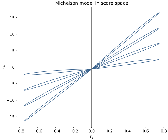
A partition into $K$ cells with probability masses $W_b$ and mean scores $\mu_b$ retains the Fisher information

$$I_{\mathrm{bin}} = \sum_{b=1}^{K} W_b\,\mu_b\mu_b^\top ,$$

a two-by-two matrix here. The first question is how to divide score space into $K$ cells if information about both parameters is to be preserved jointly. The standard answer is D-optimality:

$$\max_{q}\ \log\det I_{\mathrm{bin}} .$$

The determinant is the volume of information across all directions of score space, so maximizing it preserves information in every direction at once rather than favouring one.

6. D-optimal partition

With $K$ fixed, optimize_partition assigns the weighted score table to $K$ cells by exact single-point exchange: a node is moved between cells whenever the move increases the determinant, until no single move can.

N_BINS = 6

d_partition = sq.optimize_partition(
    scores,
    weights=weights,
    n_bins=N_BINS,
    criterion=sq.DOptimality(),
    config=sq.DExchangeConfig(seed=4),
    execution=EXECUTION,
)
d_labels = d_partition.labels

Top left: the raw score plane shaded by the six cells of the compiled D-optimal rule, the cell means, and the trajectory coloured by cell. Top right: the same cells in coordinates whitened by the binned Fisher matrix, where the rule is an ordinary nearest-mean Voronoi diagram. Bottom: the same labels pulled back to the detector coordinate, above the equal-width segments.

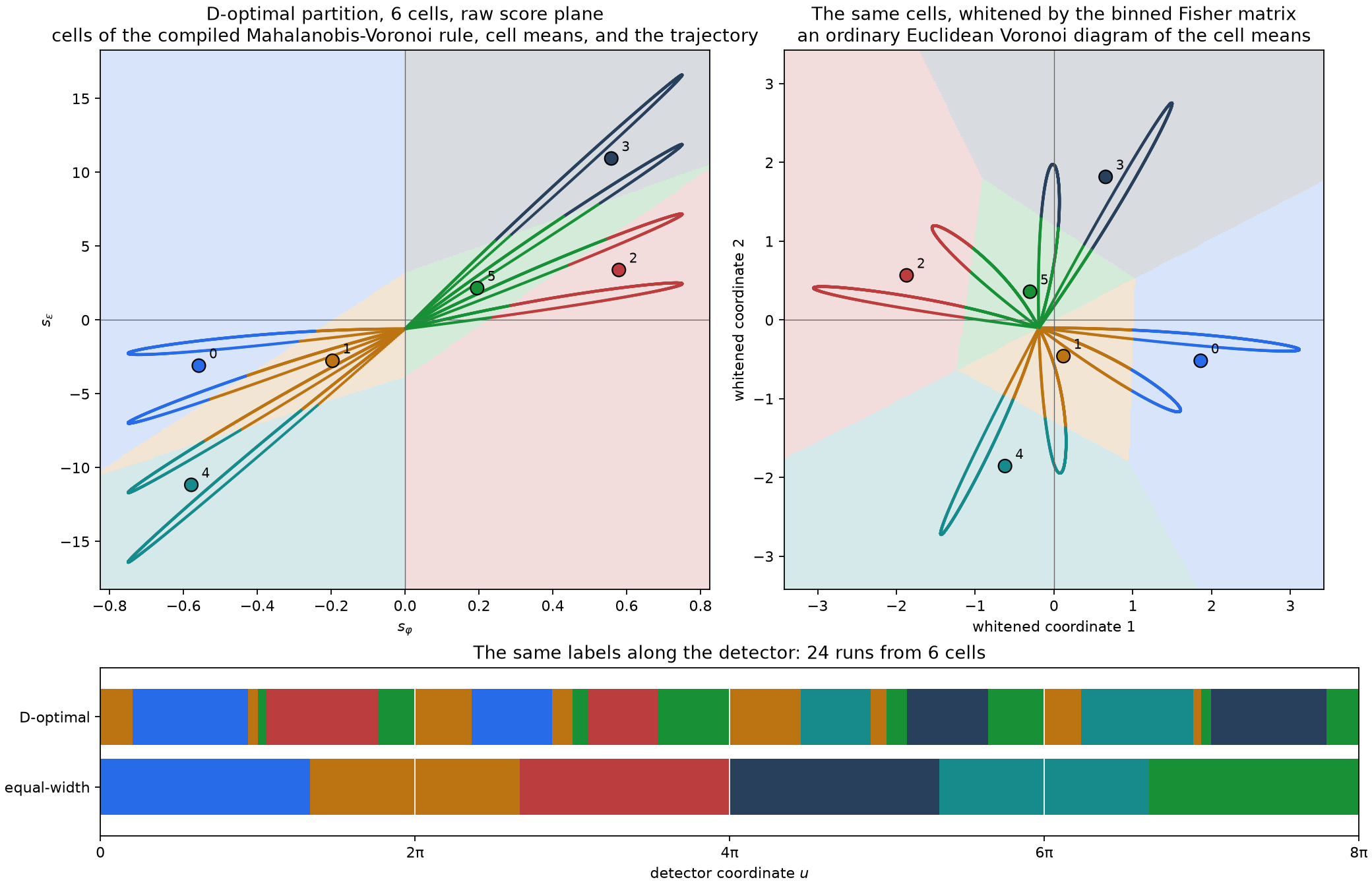
In score space the 6 cells are connected regions with straight boundaries. The raw axes are not directionally uniform: the two scores carry different units and are correlated along the trajectory, so the cells look stretched and their boundaries oblique. Whitening score space by the binned Fisher matrix removes that: in the right-hand panel the same rule is a plain nearest-mean Voronoi diagram, because an exchange-stable D-optimal partition is exactly a Voronoi partition under the inverse binned Fisher metric, and that metric is the identity in whitened coordinates. Along the detector, however, the same labels form a comb. The reason is simple: the one-dimensional score trajectory folds through the same two-dimensional cells several times. A connected cell in score space can therefore correspond to several disconnected intervals in $u$, and a brief crossing of a cell produces a narrow detector interval.

This is the geometrically clean case. An exchange-stable D-optimal partition with a nonsingular Fisher matrix is exactly a Mahalanobis–Voronoi partition of score space, with the inverse of the binned Fisher matrix as metric. The theorem and its proof are in D-optimality and exact exchange (opens in a new tab); the shading in the figure is that rule evaluated on a grid.

7. A reusable D-optimal readout

The finite optimization assigns labels only to the 8,000 grid nodes. For D-optimality, the Voronoi geometry above provides the missing inductive rule: the finite partition can be compiled into a quantizer that assigns a bin to any new score vector.

d_quantizer = d_partition.compile_quantizer(execution=EXECUTION)

new_observations = np.array([[1.0], [7.0], [15.0]])
new_scores = provider.score(new_observations, execution=EXECUTION)
new_bins_d = d_quantizer.predict_scores(new_scores, execution=EXECUTION)

The resulting readout has the form

$$u \;\longrightarrow\; s(u) \;\longrightarrow\; q\!\left(s(u)\right).$$

This distinction between a finite partition and a reusable quantizer is important. optimize_partition solves the assignment problem on a fixed weighted table; a quantizer defines a rule for new observations. For D-optimality the two are connected by the Voronoi geometry. The general distinction is discussed in Two tasks and three optimization levels (opens in a new tab).

8. Treating fringe frequency as a nuisance

The scientific question now changes. The phase $\varphi$ is the result to be reported. The frequency error $\epsilon$ is estimated only because uncertainty in it can imitate a phase shift.

Partition the binned Fisher matrix,

$$I_{\mathrm{bin}} = \begin{pmatrix} I_{\varphi\varphi} & I_{\varphi\epsilon}\\ I_{\varphi\epsilon} & I_{\epsilon\epsilon} \end{pmatrix}.$$

The information about $\varphi$ that survives estimating $\epsilon$ from the same data is the profiled phase information

$$I_{\varphi\mid\epsilon} = I_{\varphi\varphi} - \frac{I_{\varphi\epsilon}^2}{I_{\epsilon\epsilon}}.$$

The subtracted term is the part of the phase sensitivity that a change in $\epsilon$ can reproduce. In this model the two scores are strongly correlated, 0.8720 at the reference point, and profiling removes 0.7603 of the unbinned phase information before any binning.

Ordinary D-optimality treats $\varphi$ and $\epsilon$ symmetrically: it spends cells on resolving $\epsilon$ as carefully as $\varphi$. The profiled criterion $D_s$ asks instead how the $K$ cells should be spent if only $\varphi$ will be reported,

$$\max_{q}\ \log I_{\varphi\mid\epsilon}^{\mathrm{bin}} .$$

9. Optimizing for phase

Quality is measured by the fraction of the unbinned profiled phase information that a partition retains,

$$R_\varphi = \frac{I_{\varphi\mid\epsilon}^{\mathrm{bin}}} {I_{\varphi\mid\epsilon}^{\mathrm{full}}},$$

with the profiled quantity in both numerator and denominator. profiled_information_report computes exactly that ratio for any labeling.

def phase_retention(labels):
    """Profiled phase information retained, as a fraction of the unbinned value."""
    report = sq.profiled_information_report(
        scores, labels, interest=INTEREST, weights=weights, n_bins=N_BINS, execution=EXECUTION
    )
    return report.geometric_mean_retention


equal_labels = np.digitize(u, np.linspace(0.0, U_MAX, N_BINS + 1)[1:-1])
equal_width_retained = phase_retention(equal_labels)
d_retained = phase_retention(d_labels)

For a single parameter of interest, ScoreQuant can also compute a certified upper bound on the profiled information attainable with $K$ bins. We use the corresponding partition as the starting point of the $D_s$ optimization. The construction is described in Nuisance parameters and profiled Ds (opens in a new tab).

bound = sq.efficient_score_bound(
    scores, interest=INTEREST, weights=weights, n_bins=N_BINS, execution=EXECUTION
)

ds_partition = sq.optimize_partition(
    scores,
    weights=weights,
    n_bins=N_BINS,
    criterion=sq.ProfiledDOptimality(interest=INTEREST),
    config=sq.DExchangeConfig(seed=4),
    initial_labels=bound.labels,
    execution=EXECUTION,
)
ds_labels = ds_partition.labels
ds_retained = phase_retention(ds_labels)

Phase information retained, after profiling, compared across 3 binning methods

Method	Phase information retained, after profiling
Equal-width	0.2054
D-optimal	0.7995
Profiled Ds (ScoreQuant)	0.9483
Certified ceiling (reference ceiling)	0.9483

Three partitions of the same table into 6 bins. The dashed line is the certified ceiling, not a readout.

Equal-width bins retain 0.2054 of the profiled phase information. The D-optimal partition retains 0.7995: much better, but it was built to resolve both parameters. Optimizing the profiled criterion retains 0.9483.

The certified ceiling is 0.948283, compared with 0.948259 for the fitted partition. The difference is small, so there is little room for another 6-bin partition to improve the profiled phase information.

10. What changes under profiling?

Top: the trajectory coloured by the finite profiled-$D_s$ labels. Middle: the efficient score $\hat s(u)$ along the detector, coloured the same way. Bottom: the labels along the detector, drawn at true width, for the efficient-score initializer, the profiled partition and the reusable rule of the next section.

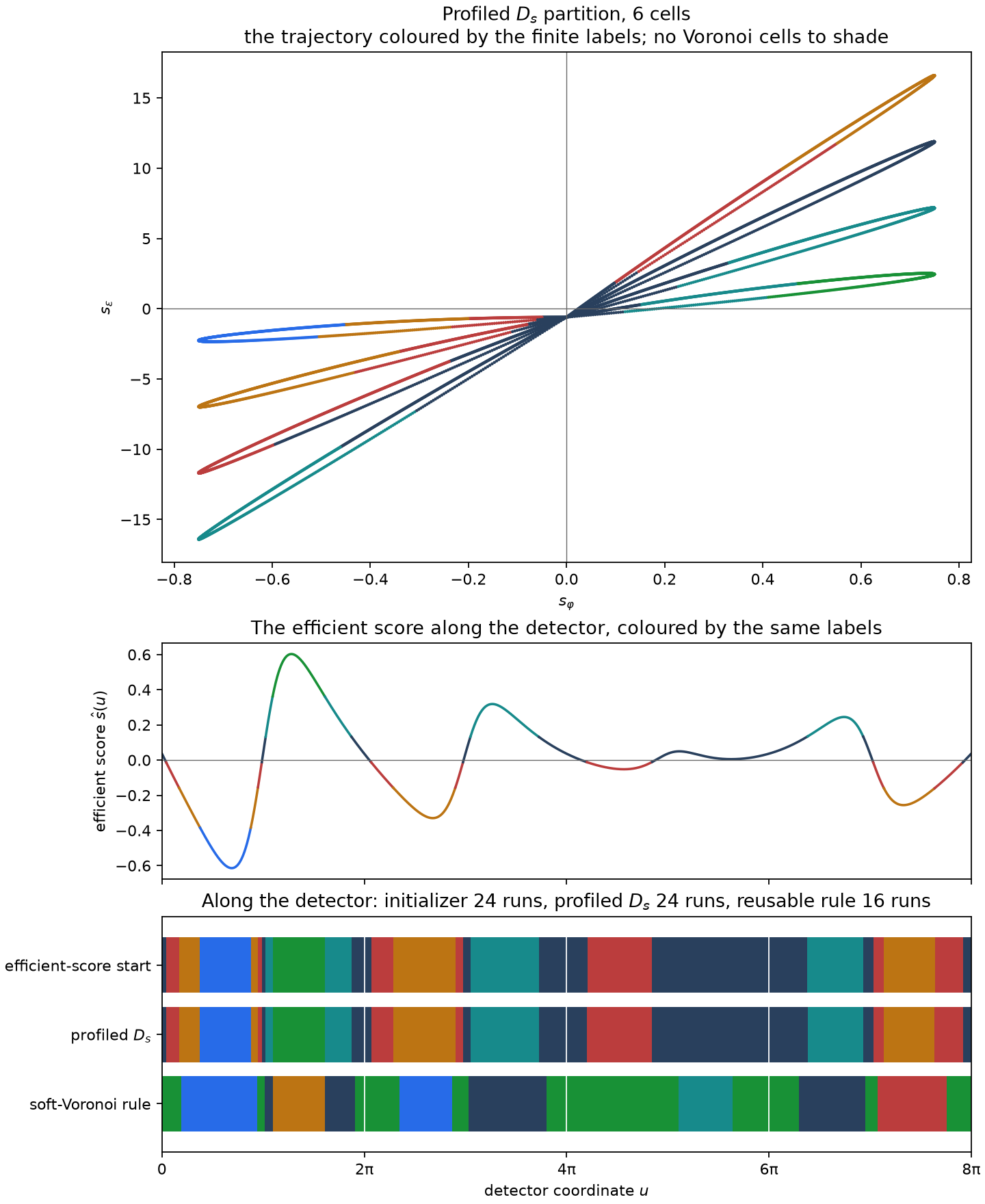
Profiling changes the structure of the solution. The ordinary D partition spends bins on resolving both score directions, while the profiled criterion concentrates on the part of the phase sensitivity that cannot be reproduced by the nuisance. The resulting labels therefore cut across the score trajectory differently.

Unlike the ordinary D case, a finite profiled-$D_s$ partition does not in general define a canonical Voronoi rule. The top panel consequently shows the finite labels on the trajectory without extending them into shaded cells. The underlying geometric distinction is discussed in A profiled optimum outside its geometry (opens in a new tab).

The narrow detector intervals are not mainly created by the exchange solver. They are already present in the efficient-score starting partition: mapping intervals of the scalar efficient score back through the oscillating detector coordinate naturally produces a fragmented comb. The final exchange changes only 0.4% of the nodes and increases retention by 1.9e-04.

Thus the extra phase information comes with a less simple detector segmentation. The next step is to ask for a reusable profiled rule rather than an unrestricted finite labeling.

11. Reusable profiled quantizer

Because the finite profiled partition has no canonical rule to compile, a deployable profiled readout is fitted directly with fit_quantizer, using the same continuous detector model and analytic score.

source = sq.IntegrationSource(
    [[0.0, U_MAX]],
    density=fringe_density,
    quadrature=sq.GaussLegendreConfig(order=256),
)

Here SoftVoronoiConfig fits a smooth score-space rule and then hardens it into a discrete $K$-bin quantizer.

ds_quantizer = sq.fit_quantizer(
    source,
    provider=provider,
    n_bins=N_BINS,
    criterion=sq.ProfiledDOptimality(interest=INTEREST),
    config=sq.SoftVoronoiConfig(seed=4, initializer_restarts=8, max_steps=1000),
    execution=EXECUTION,
)

new_bins_ds = ds_quantizer.predict_scores(new_scores, execution=EXECUTION)

The reusable rule retains 0.8794 of the profiled phase information, compared with 0.9483 for the finite partition, and uses 16 detector intervals instead of 24. This is the practical trade-off: restricting the solution to a reusable, simpler rule costs some information.

For new observations the deployment path is again

$$u \;\longrightarrow\; s(u) \;\longrightarrow\; q\!\left(s(u)\right).$$

12. Interactive bin-budget sweep

Vary the number of bins and compare equal-width, D-optimal and profiled-$D_s$ readouts. The figure shows how much profiled phase information each retains and how the corresponding labels are arranged along the detector. The button reruns the profiled fit in the browser for the selected bin budget.

Counters K

46810

Aperture readout at 6 counters

Band	Start (u)	End (u)	Counter
Profiled Ds	0.0000	0.1319	3
Profiled Ds	0.1319	0.5309	2
Profiled Ds	0.5309	1.1844	1
Profiled Ds	1.1844	2.7583	0
Profiled Ds	2.7583	2.9814	1
Profiled Ds	2.9814	3.1008	2
Profiled Ds	3.1008	3.2201	3
Profiled Ds	3.2201	3.4369	4
Profiled Ds	3.4369	5.0611	5
Profiled Ds	5.0611	5.8873	4
Profiled Ds	5.8873	6.4968	3
Profiled Ds	6.4968	7.1817	2
Profiled Ds	7.1817	9.1106	1
Profiled Ds	9.1106	9.3494	2
Profiled Ds	9.3494	9.5787	3
Profiled Ds	9.5787	11.7056	4
Profiled Ds	11.7056	13.1978	3
Profiled Ds	13.1978	15.2242	2
Profiled Ds	15.2242	20.0528	3
Profiled Ds	20.0528	21.7775	4
Profiled Ds	21.7775	22.0885	3
Profiled Ds	22.0885	22.4215	2
Profiled Ds	22.4215	23.9955	1
Profiled Ds	23.9955	24.8720	2
Profiled Ds	24.8720	25.1327	3
Plain D	0.0000	0.0031	5
Plain D	0.0031	0.6440	1
Plain D	0.6440	2.9437	0
Plain D	2.9437	3.1416	1
Plain D	3.1416	3.3018	5
Plain D	3.3018	5.5418	2
Plain D	5.5418	6.2863	5
Plain D	6.2863	7.4110	1
Plain D	7.4110	9.0195	0
Plain D	9.0195	9.4248	1
Plain D	9.4248	9.7484	5
Plain D	9.7484	11.1464	2
Plain D	11.1464	12.5695	5
Plain D	12.5695	13.9895	1
Plain D	13.9895	15.3844	4
Plain D	15.3844	15.7080	1
Plain D	15.7080	16.1132	5
Plain D	16.1132	17.7249	3
Plain D	17.7249	18.8527	5
Plain D	18.8527	19.5910	1
Plain D	19.5910	21.8309	4
Plain D	21.8309	21.9911	1
Plain D	21.9911	22.1891	5
Plain D	22.1891	24.4887	3
Plain D	24.4887	25.1327	5
Equal segments	0.0000	4.1877	0
Equal segments	4.1877	8.3786	1
Equal segments	8.3786	12.5664	2
Equal segments	12.5664	16.7541	3
Equal segments	16.7541	20.9450	4
Equal segments	20.9450	25.1327	5

The same two labellings drawn in the space they were optimized in: the score curve, four loops of growing fringe-frequency score, with each counter a colour. Profiled Ds cuts across the loops to separate the phase score; plain D spends cells resolving the loops from one another.

Phase information retained, after profiling, compared across 3 binning methods

Method	Phase information retained, after profiling
Equal segments	0.2054
Plain D	0.7995
Profiled Ds (ScoreQuant)	0.9483
Certified ceiling (reference ceiling)	0.9483

All three partitions use 6 counters on the same node table; the dashed line is the certified ceiling, not a partition you could choose. Higher is better.

Committed result0.9483Committed profiled retention at 6 counters

Fetches the same node table the study used and runs optimize_partition with the profiled criterion for phase, the exact exchange solver, seed 4, and the efficient-score-bound start -- exactly how the committed sweep row was produced. The value should agree to the digits shown; summation order can differ in the last places.

13. Summary

The score maps the detector coordinate into the space that matters for inference. Ordinary D-optimality uses that space to preserve information about both parameters and produces a clean Mahalanobis–Voronoi quantizer.

When only the phase is of interest, profiling the fringe-frequency nuisance changes the objective. With 6 bins, the retained profiled phase information rises from 0.7995 for the D-optimal readout to 0.9483 for the profiled partition.

The example also illustrates the distinction between two ScoreQuant tasks: optimizing labels on a finite weighted table and fitting a reusable rule for new observations. For ordinary D the first can be compiled into the second; for profiled $D_s$ the reusable rule must be fitted explicitly.

Where the theory is. The exchange algorithm, the Voronoi theorem and the compile bridge: D-optimality and exact exchange (opens in a new tab). The profiled criterion, the efficient score and the certified ceiling: Nuisance parameters and profiled Ds (opens in a new tab). The two tasks: Two tasks and three optimization levels (opens in a new tab).