Part V: Performance, Accuracy, and Integration
This part summarizes where the ChESS detector stands today on accuracy and speed (measured on a MacBook Pro M4), how well it matches classic OpenCV detectors on a stereo calibration dataset, how to interpret the traces we emit, and how to integrate the detector into larger pipelines.
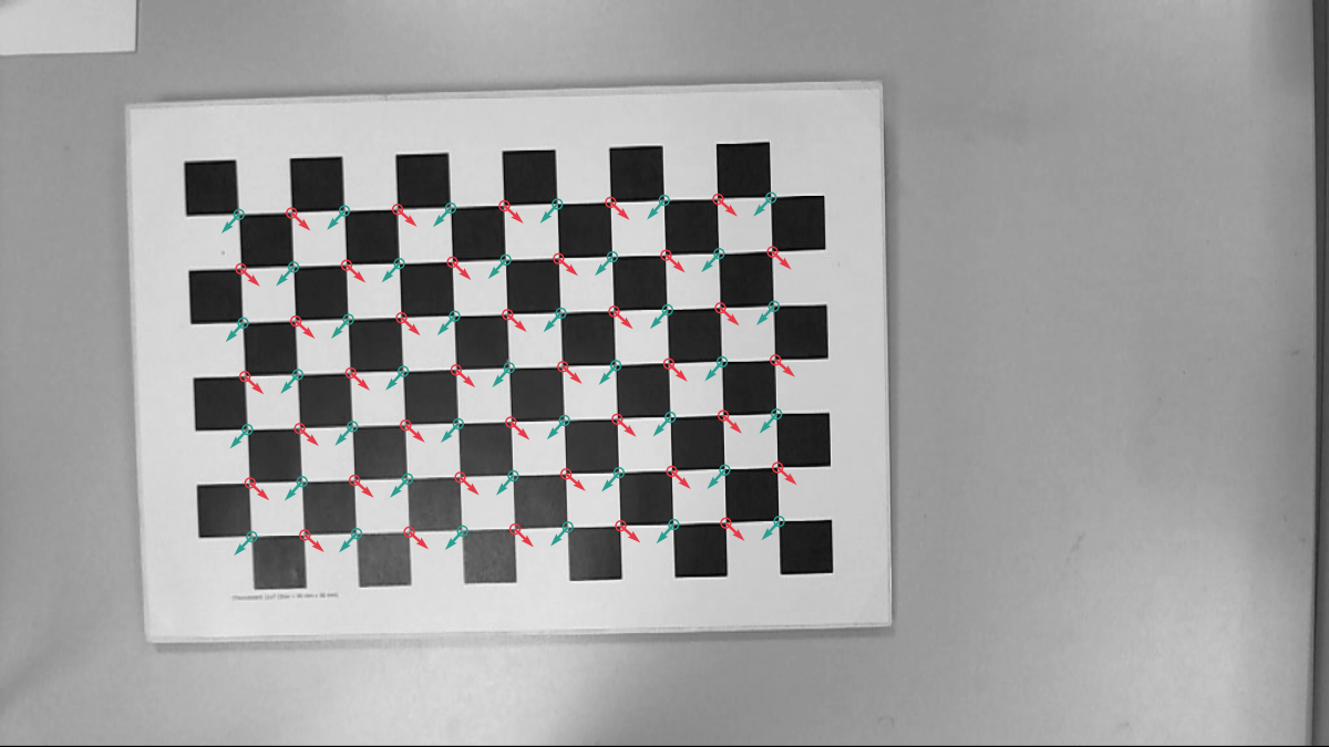
We took three test images as use cases:
- A clear 1200x900 image of a chessboard calibration target:
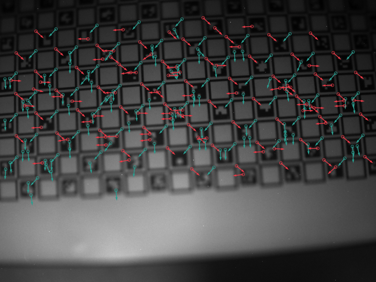
- A 720x540 image of a ChArUco target with not perfect focus:
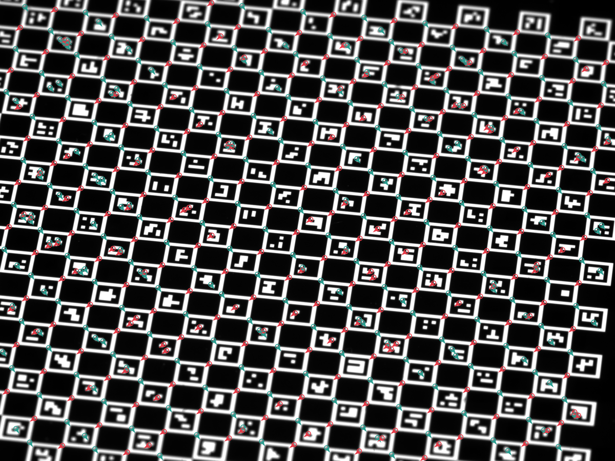
- A 2048x1536 image of another ChArUco calibration target:
We traced the ChESS detector for each of these images, and the results are discussed in this part. The first image was also used to compare with OpenCV Harris features and the findChessboardCornersSB function. For accuracy, we additionally evaluated the detector on a 2×20‑frame stereo dataset (77 corners per frame).
5.1 Performance
The tests below were run on a MacBook Pro M4 (release build). Absolute numbers will vary on your hardware, but the relative behavior between configurations is quite stable.
Per‑image timings (ms, averaged over 10 runs; see book/src/perf.txt and testdata/out/perf_report.json for the full breakdown):
| Config | Features | small | mid | large |
|---|---|---|---|---|
| Single‑scale | none | 3.01 | 4.46 | 26.02 |
| Single‑scale | simd | 1.29 | 1.74 | 10.00 |
| Single‑scale | rayon | 1.14 | 1.41 | 6.63 |
| Single‑scale | simd+rayon | 0.92 | 1.15 | 5.34 |
| Multiscale (3 l) | none | 0.63 | 0.70 | 4.87 |
| Multiscale (3 l) | simd | 0.40 | 0.42 | 2.77 |
| Multiscale (3 l) | rayon | 0.48 | 0.52 | 1.94 |
| Multiscale (3 l) | simd+rayon | 0.49 | 0.54 | 1.59 |
Highlights from the timing profiles on small/mid/large images:
- Multiscale is the clear winner for speed and robustness.
- Large image: best total ≈ 1.6 ms with
simd+rayon(vs ≈4.9 ms with no features, ≈1.9 ms withrayononly). - Mid: best total ≈ 0.42 ms with
simdalone (rayon adds a bit of overhead at this size). - Small: best total ≈ 0.40 ms with
simd. - Breakdown: refine dominates (0.1–3 ms depending on seeds); coarse_detect sits around 0.08–0.75 ms; merge is negligible.
- Large image: best total ≈ 1.6 ms with
- Single-scale is slower across the board:
- Large: ≈26 ms, mid: ≈4.5 ms, small: ≈3.0 ms. Use when you need maximal stability and can tollerate some performance drawback.
- Feature guidance:
- Enable simd by default; it’s the dominant win on all sizes (although, it requires nightly RUST).
- Add rayon for large inputs (wins on the largest image, minor cost on small/mid).
5.2 Accuracy vs OpenCV
The OpenCV cornerHarris gives the following result:
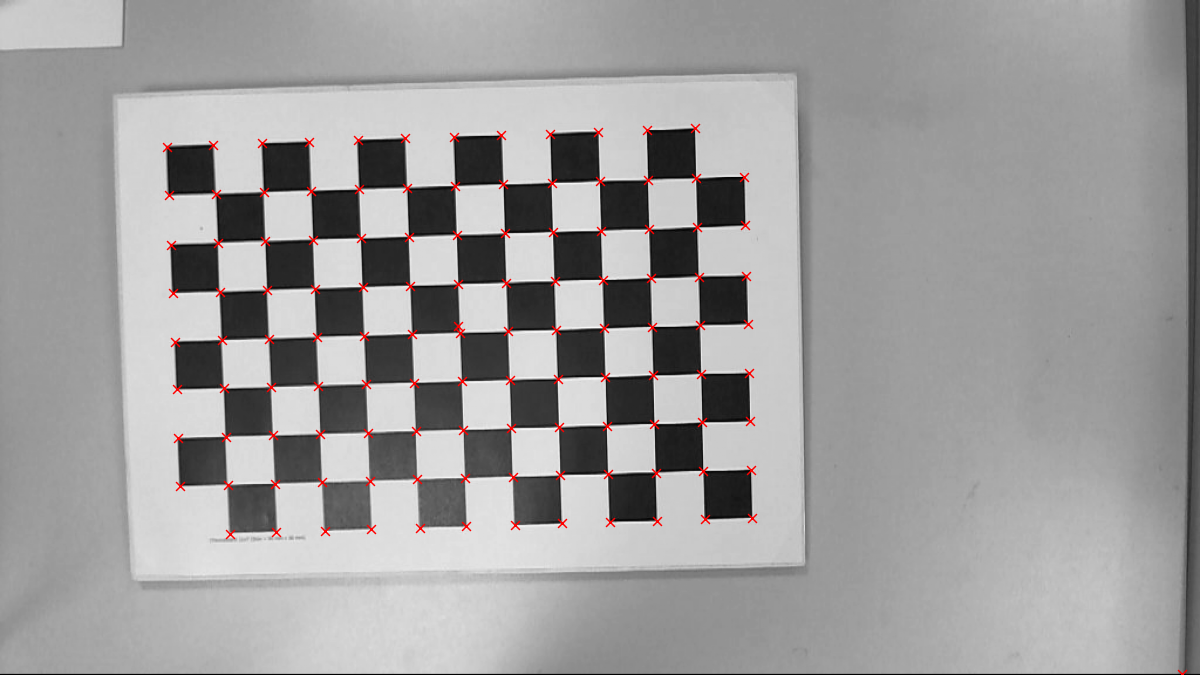
Here is the result of the OpenCV findChessboardCornersSB function:
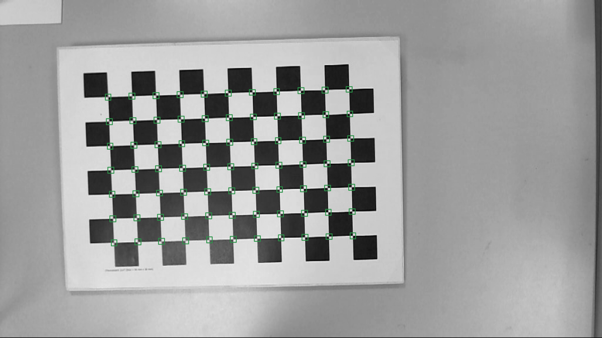
Harris pixel-level feature detection took 3.9 ms. The final result is obtained by using the cornerSubPix and manual merge of duplicates. Chessboard detection took about 115 ms. The ChESS detector is much faster as is evident from the previous section. Also, it provides corner orientation that can be handy for a grid reconstruction.
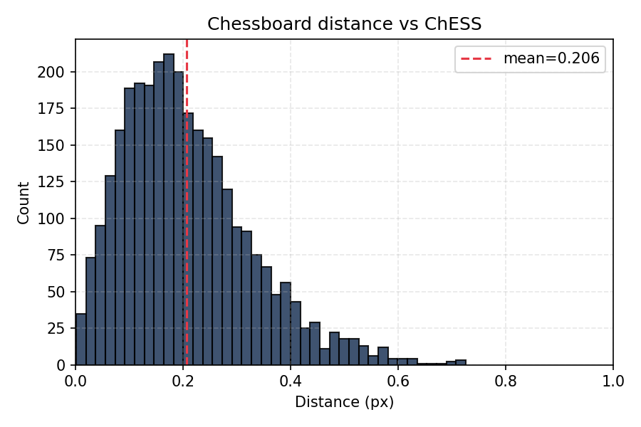
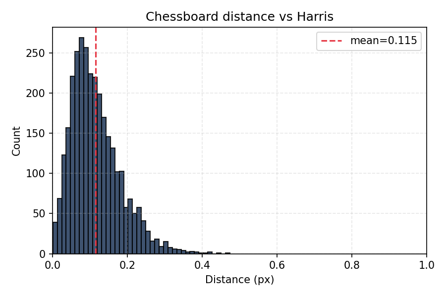
Below we compare the ChESS corners location with the two classical references. We took all images from the Chessboard Pictures for Stereocamera Calibration public repository as input. Below are distributions of pairwise distances between corresponding features:
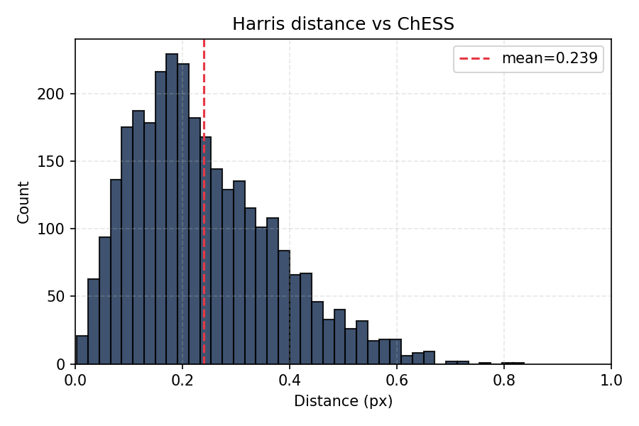
- Harris vs ChESS: 0.24 pix
- Chessboard vs ChESS: 0.21 pix
- Harris vs Chessboard: 0.12 pix
It is important that the offsets are not biased:
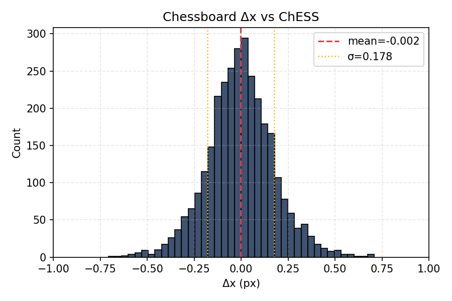
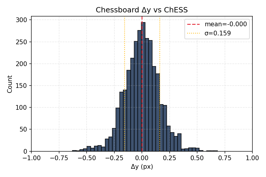
Mean values are much smaller than standard deviation.
5.3 ML refiner (synthetic evaluation)
The ML refiner was trained and evaluated on synthetic corner patches
generated by the tooling under tools/ml_refiner:
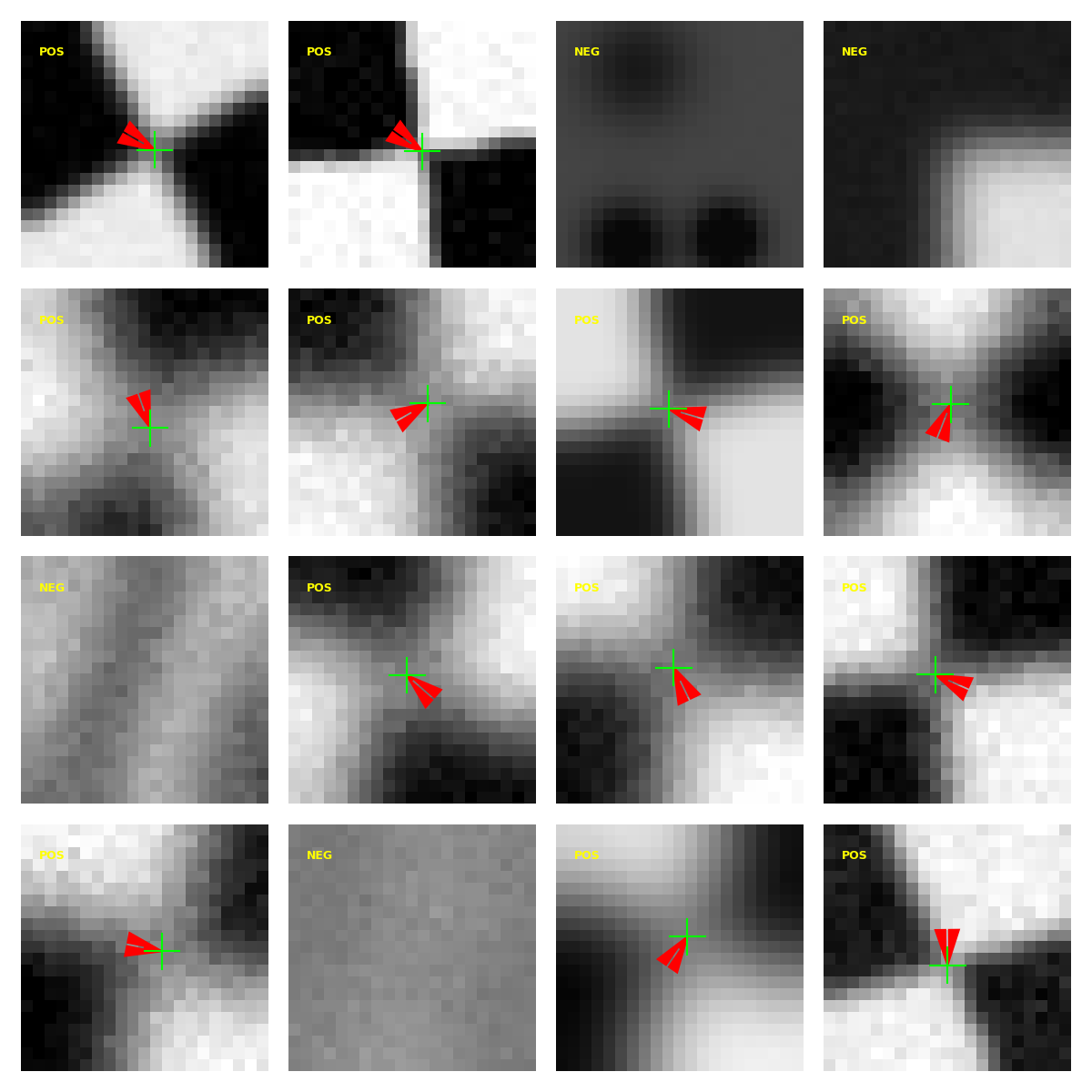
The generator renders a
canonical chessboard corner, applies random homographies, blur, and noise, then
labels each patch with a subpixel offset (dx, dy) and a confidence score
derived from the distortion severity. The model predicts [dx, dy, conf_logit]
on normalized patches (uint8 / 255.0). The current Rust path ignores the
confidence output and applies offsets directly (confidence is used during
training/evaluation only).
Training and evaluation steps:
- Generate synthetic datasets with
tools/ml_refiner/synth/generate_dataset.py. - Train the refiner with
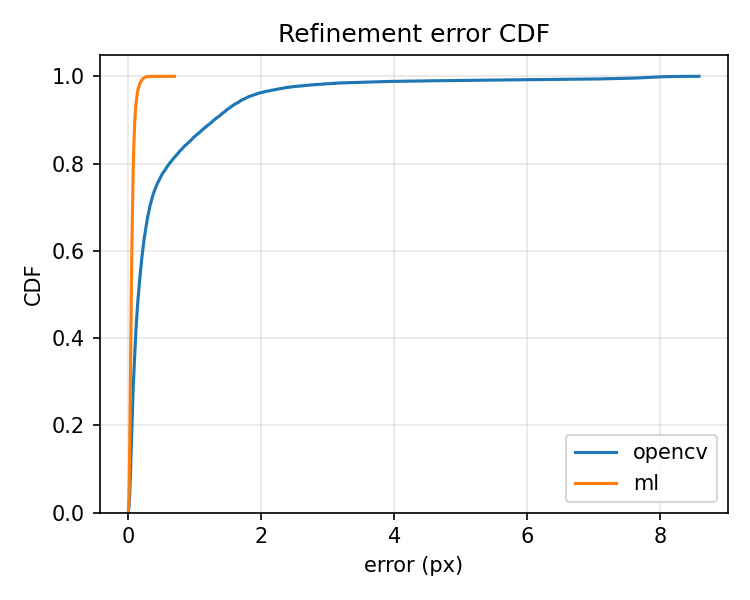
tools/ml_refiner/train.py(regression on positives, confidence on all samples). - Compare to OpenCV
cornerSubPixviatools/ml_refiner/eval/compare_opencv.py, which writes a JSON summary and plots for CDF and error vs noise/blur severity.
Updated results (synthetic data):
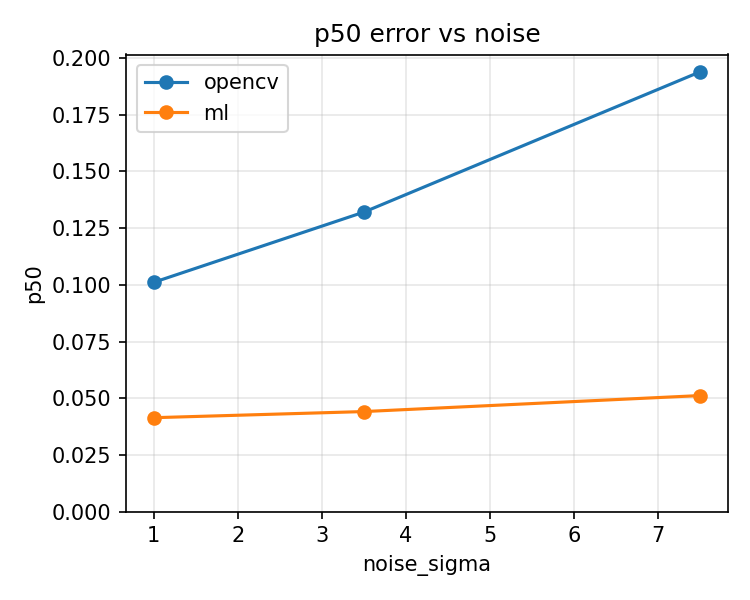
Numeric aggregates live in book/src/img/ml_summary.json (exported by the
evaluation scripts).
On this synthetic benchmark, the ML refiner shows substantially tighter error
distributions than OpenCV cornerSubPix, especially under noise and blur.
This does not yet guarantee real-world performance; realistic datasets still
need to be tested.
Timing note (single-scale on testimages/mid.png, 77 corners):
- Classic refinement: ~0.6 ms
- ML refinement: ~23.5 ms
The ML path trades speed for precision, so use it selectively (e.g., for off-line calibration or when accuracy is paramount).
5.4 Tracing and diagnostics
- Build with the
tracingfeature (the perf script does this) to emit INFO-level JSON spans. - Key spans now covered in both paths:
find_chess_corners(total)single_scale(single-path body)coarse_detect(coarse response + detection)refine(per-seed refinement, includesseedscount)merge(duplicate suppression)build_pyramid(pyramid construction)ml_refiner(ML refinement span + timing event when enabled)
- Parsing:
tools/trace/parser.pyextracts the spans above;perf_report.jsonis produced bytools/perf_bench.py, and accuracy overlays/timings come fromtools/accuracy_bench.py. - Use
--json-traceon the CLI (or run viaperf_bench.py) to capture traces; visualize or aggregate with your preferred JSON tools.
5.5 Integration patterns
- Real-time loops: reuse
PyramidBuffersviafind_chess_corners_buff; prefer multiscale + simd, add rayon for larger frames. Keepmerge_radiusmodest (2–3 px) to avoid duplicate corners without throwing away tight clusters. - Calibration/pose: the accuracy report shows sub-pixel consistency; feed detected corners directly into calibration routines. Use the accuracy histograms to validate new camera data.
- Diagnostics in the field: capture a short trace with
--json-traceand inspectrefine_seedsand span timings; spikes usually indicate harder scenes (more seeds) or contention (misconfigured features). - Reproducibility: keep generated reports under
testdata/out/; rerunaccuracy_bench.py --batchandperf_bench.pyafter algorithm or config changes, and drop updated plots into docs for before/after comparisons.