
Part I: Orientation
Part of the vitavision.dev computer-vision atlas. Self-contained algorithm overviews live at vitavision.dev/atlas/chess-corners and vitavision.dev/atlas/duda-radon-corners; this book is the implementation reference for the Rust workspace.
1.1 What the library does
chess-corners-rs detects the corners of a chessboard pattern — the
X-junctions where four alternating dark/bright cells meet — to
sub-pixel precision. It is the kind of detector that sits at the
front of a camera calibration, pose estimation, or AR alignment
pipeline.
Two independent detectors and five subpixel refiners live behind a single configuration type:
- ChESS response detector — a ring-based kernel from Bennett & Lasenby (2014). This is the default and the fastest preset in the measured clean-image benchmark. Covered in Part III; atlas overview at vitavision.dev/atlas/chess-corners.
- Radon response detector — a ray-based kernel from Duda & Frese (2018). Added for cases where the ChESS ring does not produce enough seeds, especially the small-cell, blur, and low-contrast fixtures in this repository. Covered in Part IV; atlas overview at vitavision.dev/atlas/duda-radon-corners.
Both produce the same CornerDescriptor output, and both feed the
same multiscale pipeline.
Once a detector has produced integer-pixel seeds, one of five
subpixel refiners brings the coordinates under a pixel:
CenterOfMass, Förstner, SaddlePoint, RadonPeak, or an
ONNX-backed ML refiner. Each is selected through the active
strategy’s refiner field. The refiners are described in
Part V and benchmarked in
Part VIII.
The same DetectorConfig drives a Rust API, a Python package, a
browser WebAssembly package, and a CLI. They call the same Rust
detector pipeline and use the same configuration schema.
1.2 Typical use cases
- Camera calibration (mono, stereo, or multi-camera) with printed or screen-displayed chessboard targets.
- Pose estimation of calibration rigs and fixtures.
- Robotics and AR setups where a chessboard is a temporary alignment target.
- Offline evaluation of external calibration pipelines: the detectors here are deterministic and independent of OpenCV.
Compared with other corner pipelines:
- Versus generic corner detectors (Harris, Shi–Tomasi, FAST): both detectors here are specialized for chessboard X-junctions and reject edges, blobs, and texture that generic detectors accept.
- Versus ID-based markers (AprilTag, ArUco): this library detects unlabeled grid corners. It does not decode an ID, so you need to know the board layout separately.
1.3 Workspace layout
The library is split across six crates; three are user-facing and three are implementation detail you only need if you want to go below the facade.
┌─ chess-corners-py      (PyO3 bindings, pip package: chess-corners)
├─ chess-corners-wasm    (wasm-bindgen, npm package: @vitavision/chess-corners)
│                        ▲
│                        │
├─ chess-corners         (high-level Rust API, CLI, multiscale pipeline)
│                        ▲
│                        │
├─ chess-corners-core    (low-level algorithms: ChESS + Radon detectors,
│                         refiners, descriptors)
│
├─ box-image-pyramid     (standalone u8 pyramid builder, fully
│                         independent — no chess-specific coupling)
│
└─ chess-corners-ml      (optional ONNX refiner; gated behind
                          `ml-refiner` feature)
Layering rules enforced by CI:
chess-corners-coredoes not depend onchess-corners.box-image-pyramidhas no chess-specific code — it is a reusable grayscale pyramid builder that happens to be used here.- Algorithms go in
chess-corners-core; the facade crate adds the publicDetectorConfigtype, CLI, multiscale wiring, and feature gates.
Support directories:
config/— example CLI JSON configs.testdata/— sample images used by tests, examples, and book plots.tools/— Python scripts for plotting, benchmarking, and the ML refiner training pipeline.docs/— design notes, proposals, and backlog.book/— this book (mdBook source underbook/src/).
1.4 The CornerDescriptor output
Every detector in the workspace returns Vec<CornerDescriptor>.
The type lives in chess-corners-core and is re-exported by the
facade. Fields:
| Field | Type | Meaning |
|---|---|---|
x, y | f32 | Subpixel position in input image pixels. |
response | f32 | Raw detector response at the peak. Scale is detector-specific. |
contrast | f32 (≥ 0) | Bright/dark amplitude from the ring intensity fit (gray levels). |
fit_rms | f32 (≥ 0) | RMS residual of that fit (gray levels). |
axes[0, 1] | [AxisEstimate; 2] | The two local grid axis directions, each with a 1σ angular uncertainty. |
The two axes are not assumed orthogonal — projective warp or
lens distortion tilts the sectors independently, and the fit
recovers both directions. Polarity convention:
axes[0].angle ∈ [0, π), axes[1].angle ∈ (axes[0].angle, axes[0].angle + π),
with the CCW arc from axis 0 to axis 1 crossing a dark sector. Full
details and the fit math are in
Part III §3.4.
1.5 Where to go next
- To run the detector on an image: Part II.
- To understand the ChESS response: Part III.
- To understand the Radon response: Part IV.
- To pick a refiner: Part V for algorithms, Part VIII for measurements.
- Orientation methods (
RingFit/DiskFit): Part VI. - Multiscale pipeline and pyramid tuning: Part VII.
- To contribute: Part IX.
Rust API documentation builds alongside this book and is published at the same site:
chess-cornersAPI referencechess-corners-coreAPI referencebox-image-pyramidAPI referencechess-corners-mlAPI reference
1.6 Installation and features
Rust
[dependencies]
chess-corners = "0.11"
image = "0.25"      # if you want GrayImage integration
Feature flags on the chess-corners facade:
| Feature | Effect |
|---|---|
image | Default. image::GrayImage convenience entry points. |
rayon | Parallelize response computation and multiscale refinement over cores. |
simd | Portable SIMD for the ChESS kernel. Nightly only. |
par_pyramid | SIMD / Rayon acceleration inside the pyramid downsampler. |
tracing | Structured tracing spans for the detector pipeline. |
ml-refiner | Enable the ONNX-backed refiner (chess-corners-ml dependency). |
cli | Build the chess-corners binary. |
All feature combinations produce the same numerical results; features only affect performance and observability.
Python
python -m pip install chess-corners
JavaScript / WebAssembly
wasm-pack build crates/chess-corners-wasm --target web
# installs an npm package: chess-corners-wasm
CLI
cargo run -p chess-corners --release --bin chess-corners -- \
    run config/chess_cli_config_example.json
Every surface consumes the same DetectorConfig JSON schema. Examples
live under config/. The next part walks through the public API in
all four surfaces.
Part II: Using the library
This chapter is a walk through the public API on every binding target. Code-first; algorithms are covered in Part III (ChESS), Part IV (Radon), and Part V (refiners).
2.1 Configuration shape
DetectorConfig has one place for every knob. Cross-cutting fields
sit at the top level; detector-specific fields are nested inside the
active strategy variant.
| Top-level field | Type |
|---|---|
strategy | DetectionStrategy::Chess(ChessConfig) or DetectionStrategy::Radon(RadonConfig) — selects the detector and carries its tuning. |
threshold | Threshold::Absolute(f32) or Threshold::Relative(f32). Absolute(0.0) is the ChESS paper’s R > 0 contract; Relative(0.01) is the Radon preset default. |
multiscale | MultiscaleConfig::SingleScale or MultiscaleConfig::Pyramid { levels, min_size, refinement_radius }. Honoured by both detectors. |
upscale | UpscaleConfig::Disabled or UpscaleConfig::Fixed(factor) (factor ∈ {2, 3, 4}). Pre-pipeline bilinear upscaling for low-resolution inputs. |
orientation_method | OrientationMethod::RingFit (default) or DiskFit. Drives the two-axis descriptor fit on both detectors. |
merge_radius | Duplicate-suppression distance (base-image pixels) for the final cross-scale merge step. |
Inside ChessConfig:
| Field | Meaning |
|---|---|
ring | ChessRing::Canonical (r=5, paper default) or ChessRing::Broad (r=10, wider support window). The single source of truth for “broad” detection. |
descriptor_ring | DescriptorRing::FollowDetector (default), Canonical, or Broad. Lets you sample the descriptor ring at a different radius than the detector. |
nms_radius | Non-maximum-suppression window half-radius, in input-image pixels. |
min_cluster_size | Minimum positive-response neighbours inside the NMS window. |
refiner | ChessRefiner::CenterOfMass(_), Forstner(_), SaddlePoint(_), or Ml (with ml-refiner). Each variant carries its own tuning struct. |
Inside RadonConfig:
| Field | Meaning |
|---|---|
ray_radius | Half-length of each ray (working-resolution pixels). Paper default at image_upsample = 2 is 4. |
image_upsample | 1 (no supersample) or 2 (paper default). Values ≥ 3 are clamped to 2. |
response_blur_radius | Half-size of the box blur applied to the response map. 0 disables blurring. |
peak_fit | PeakFitMode::Parabolic or Gaussian for the 3-point subpixel refinement. |
nms_radius | NMS half-radius, in working-resolution pixels. |
min_cluster_size | Minimum positive-response neighbours inside the NMS window. |
refiner | RadonRefiner::RadonPeak(_) or CenterOfMass(_). |
Four presets cover the common cases:
| Preset | Detector | Scale |
|---|---|---|
DetectorConfig::chess() | ChESS | Single-scale |
DetectorConfig::chess_multiscale() | ChESS | 3-level pyramid |
DetectorConfig::radon() | Radon | Single-scale |
DetectorConfig::radon_multiscale() | Radon | 3-level pyramid |
Three guarantees follow from this shape:
- One place per knob.
cfg.strategy.chess.ring = ChessRing::Broadis the only way to request the wider ChESS sampling ring. There is no parallel top-level “broad” flag. - Per-detector refiners.
ChessRefinerlists only the refiners that operate on ChESS output;RadonRefinerlists only those that operate on Radon output. AChessRefiner::RadonPeakmismatch is unrepresentable. - Enum-with-payload everywhere a knob has an “on/off + tuning”
shape.
Threshold,MultiscaleConfig,UpscaleConfig, and both refiner enums share the same encoding, so the JSON shape and the binding surface stay symmetric across all of them.
2.2 Rust
Add the facade crate:
[dependencies]
chess-corners = "0.11"
image = "0.25"          # optional, for GrayImage integration
2.2.1 Single-scale ChESS detection from an image file
use chess_corners::{Detector, DetectorConfig};
use image::io::Reader as ImageReader;

fn main() -> Result<(), Box<dyn std::error::Error>> {
    let img = ImageReader::open("board.png")?.decode()?.to_luma8();

    let cfg = DetectorConfig::chess();  // ChESS detector, defaults
    let mut detector = Detector::new(cfg)?;
    let corners = detector.detect(&img)?;

    println!("found {} corners", corners.len());
    Ok(())
}
corners is a Vec<CornerDescriptor> with subpixel positions and
per-corner intensity-fit metadata (Part I §1.4).
2.2.2 Radon detector instead of ChESS
#![allow(unused)]
fn main() {
use chess_corners::{Detector, DetectorConfig};

let cfg = DetectorConfig::radon();           // Radon detector, paper defaults
let mut detector = Detector::new(cfg)?;
let corners = detector.detect(&img)?;
}
DetectorConfig::radon() builds a DetectionStrategy::Radon(RadonConfig)
with the paper’s published defaults. The output type is the same
Vec<CornerDescriptor>.
Try Radon when ChESS’s 16-sample ring does not seed enough corners, especially on the small-cell, blur, and low-contrast cases covered by the repository tests. For throughput, ChESS is faster in the measured fixtures; see Part IV §4.5.
2.2.3 Swapping the subpixel refiner
#![allow(unused)]
fn main() {
use chess_corners::{ChessRefiner, DetectorConfig};

let cfg = DetectorConfig::chess_multiscale()
    .with_chess(|c| c.refiner = ChessRefiner::forstner());
}
Each refiner variant carries its tuning struct inline:
#![allow(unused)]
fn main() {
use chess_corners::{ChessRefiner, ForstnerConfig};

let f = ForstnerConfig {
    max_offset: 2.0,
    ..ForstnerConfig::default()
};
let refiner = ChessRefiner::Forstner(f);
}
The Radon strategy uses RadonRefiner instead — see
Part V for which refiners apply to which detector
and why.
2.2.4 Raw buffer API
If your pixels come from a camera SDK, FFI, or GPU pipeline, skip
the image crate and feed a packed &[u8]:
#![allow(unused)]
fn main() {
use chess_corners::{Detector, DetectorConfig, Threshold};

fn detect(img: &[u8], width: u32, height: u32) -> Result<(), chess_corners::ChessError> {
    let mut cfg = DetectorConfig::chess()
        .with_threshold(Threshold::Relative(0.2));

    let mut detector = Detector::new(cfg)?;
    let corners = detector.detect_u8(img, width, height)?;
    println!("found {} corners", corners.len());
    Ok(())
}
}
Requirements:
imgiswidth * heightbytes, row-major.0is black,255is white.
If your buffer has a stride or is interleaved RGB, copy the luminance channel to a packed buffer first. The facade does not resample stride; the only supported layout is tightly packed.
2.2.5 Inspecting corners
#![allow(unused)]
fn main() {
for c in &corners {
    println!(
        "({:.2}, {:.2})  response={:.1}  axes=({:.2}, {:.2}) rad",
        c.x, c.y, c.response,
        c.axes[0].angle, c.axes[1].angle,
    );
}
}
The axes field gives two directions, both in radians; they are
not assumed orthogonal. c.axes[0].sigma and c.axes[1].sigma are
1σ angular uncertainties. See
Part III §3.4
for the fit and the polarity convention.
2.3 Python
Install from PyPI:
python -m pip install chess-corners
import numpy as np
import chess_corners

img = np.zeros((128, 128), dtype=np.uint8)

cfg = chess_corners.DetectorConfig.chess_multiscale()
cfg.threshold = chess_corners.Threshold.relative(0.15)

# Nested getters return the live shared object, so direct attribute
# assignment propagates back to `cfg` — no rebuild needed:
cfg.strategy.chess.refiner = chess_corners.ChessRefiner.forstner()

detector = chess_corners.Detector(cfg)
corners = detector.detect(img)
print(corners.shape)   # (N, 9)
Detector(cfg).detect(image) accepts a 2D uint8 array shaped
(H, W) and returns a float32 array with stride 9 per corner:
[x, y, response, contrast, fit_rms,
 axis0_angle, axis0_sigma, axis1_angle, axis1_sigma]
The Python DetectorConfig mirrors the Rust type field-for-field and
supports to_dict(), from_dict(), to_json(), from_json(),
pretty(), and print(). The factory methods are chess(),
chess_multiscale(), radon(), and radon_multiscale().
Tagged enum classes follow the same idiom across the board: read
cfg.threshold.kind / cfg.threshold.value, build a new one with
Threshold.absolute(...) or Threshold.relative(...). The same
pattern applies to MultiscaleConfig.single_scale() /
.pyramid(...), UpscaleConfig.disabled() / .fixed(k),
ChessRefiner.center_of_mass(...) / .forstner(...) /
.saddle_point(...) / .ml(), and RadonRefiner.radon_peak(...) /
.center_of_mass(...).
Nested getters (cfg.strategy, cfg.strategy.chess, cfg.threshold,
cfg.multiscale, …) all return the live shared object held by the
parent — direct attribute assignment is enough:
cfg.strategy.chess.refiner = chess_corners.ChessRefiner.forstner()
cfg.strategy.chess.ring = chess_corners.ChessRing.BROAD
For chainable single-expression edits, use the with_chess(**kwargs) /
with_radon(**kwargs) builders, which return a new config with only
the named fields replaced:
cfg = cfg.with_chess(
    refiner=chess_corners.ChessRefiner.forstner(),
    ring=chess_corners.ChessRing.BROAD,
)
The Radon strategy is selected the same way:
cfg = chess_corners.DetectorConfig.radon()
If the wheel was built with ml-refiner, the ML pipeline is reached
through the same Detector(cfg).detect(img) call once the active ChESS
refiner is the ml variant:
cfg.strategy.chess.refiner = chess_corners.ChessRefiner.ml()
2.4 JavaScript / WebAssembly
Build the wasm package from source:
wasm-pack build crates/chess-corners-wasm --target web
Or consume the published npm package @vitavision/chess-corners. Usage
from a web app:
import init, {
  ChessDetector,
  ChessConfig,
  ChessRefiner,
  ChessRing,
  DetectionStrategy,
  DetectorConfig,
  ForstnerConfig,
  MultiscaleConfig,
  Threshold,
} from '@vitavision/chess-corners';

await init();

// Build a typed configuration tree.
const cfg = DetectorConfig.chessMultiscale();
cfg.threshold = Threshold.relative(0.15);
cfg.multiscale = MultiscaleConfig.pyramid(3, 128, 3); // levels, minSize, refinementRadius

const chess = new ChessConfig();
chess.ring = ChessRing.Broad;
chess.refiner = ChessRefiner.withForstner(new ForstnerConfig());
cfg.strategy = DetectionStrategy.fromChess(chess);

const detector = ChessDetector.withConfig(cfg);

// From a canvas (webcam frame, loaded image, etc.)
const imageData = ctx.getImageData(0, 0, width, height);
const corners = detector.detect_rgba(imageData.data, width, height);

// corners is Float32Array, stride 9 per corner — same layout as Python.
for (let i = 0; i < corners.length; i += 9) {
    console.log(`(${corners[i].toFixed(2)}, ${corners[i + 1].toFixed(2)})`);
}

// Raw response map, for heatmap visualisation (opt-in diagnostic).
const response = detector.diagnostics_response_rgba(imageData.data, width, height);
ChessDetector reads and writes its full configuration through the
typed tree — detector.getConfig() returns an independent
DetectorConfig snapshot and detector.applyConfig(cfg) commits
edits. The factory functions on the tagged classes follow the same
with* idiom: ChessRefiner.withForstner(cfg),
ChessRefiner.withCenterOfMass(cfg),
ChessRefiner.withSaddlePoint(cfg), RadonRefiner.withRadonPeak(cfg),
RadonRefiner.withCenterOfMass(cfg), MultiscaleConfig.singleScale(),
MultiscaleConfig.pyramid(levels, minSize, refinementRadius), UpscaleConfig.disabled(),
UpscaleConfig.fixed(factor).
2.5 CLI
cargo run -p chess-corners --release --bin chess-corners -- \
    run config/chess_cli_config_example.json
The CLI:
- Loads the image at the config’s
imagefield. - Picks single-scale or multiscale from the top-level
multiscalefield. - Picks ChESS or Radon from
strategy(the top-level variant). - Picks the refiner from the strategy’s nested
refinerblock. - Writes a JSON summary and a PNG overlay with one mark per corner.
The JSON config is the same DetectorConfig schema as the Rust and
Python APIs, wrapped in a CLI envelope that adds image,
output_json, output_png, log_level, and ml:
{
  "image": "testimages/mid.png",
  "strategy": {
    "chess": {
      "ring": "canonical",
      "descriptor_ring": "follow_detector",
      "nms_radius": 2,
      "min_cluster_size": 2,
      "refiner": { "center_of_mass": { "radius": 2 } }
    }
  },
  "threshold": { "absolute": 0.0 },
  "multiscale": "single_scale",
  "upscale": "disabled",
  "orientation_method": "ring_fit",
  "merge_radius": 3.0,
  "output_json": null,
  "output_png": null,
  "log_level": "info"
}
Example configs under config/:
chess_algorithm_config_example.json— just the algorithm fields, the pureDetectorConfigshape shared with the Rust and Python APIs.chess_cli_config_example.json— algorithm fields plus CLI I/O envelope.chess_cli_config_example_ml.json— same, with the ML refiner enabled. Requires a binary built with--features ml-refiner.
Per-flag overrides (applied on top of the JSON):
--threshold-absolute <v>/--threshold-relative <f>--chess-ring canonical|broad--descriptor-ring follow_detector|canonical|broad--chess-refiner center_of_mass|forstner|saddle_point--radon-refiner radon_peak|center_of_mass--pyramid-levels <n>(1 = single-scale)--upscale-factor 0|2|3|4
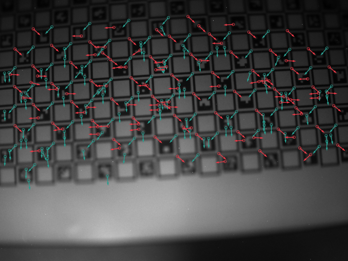
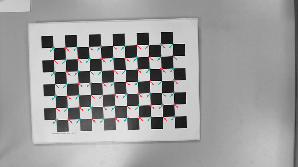
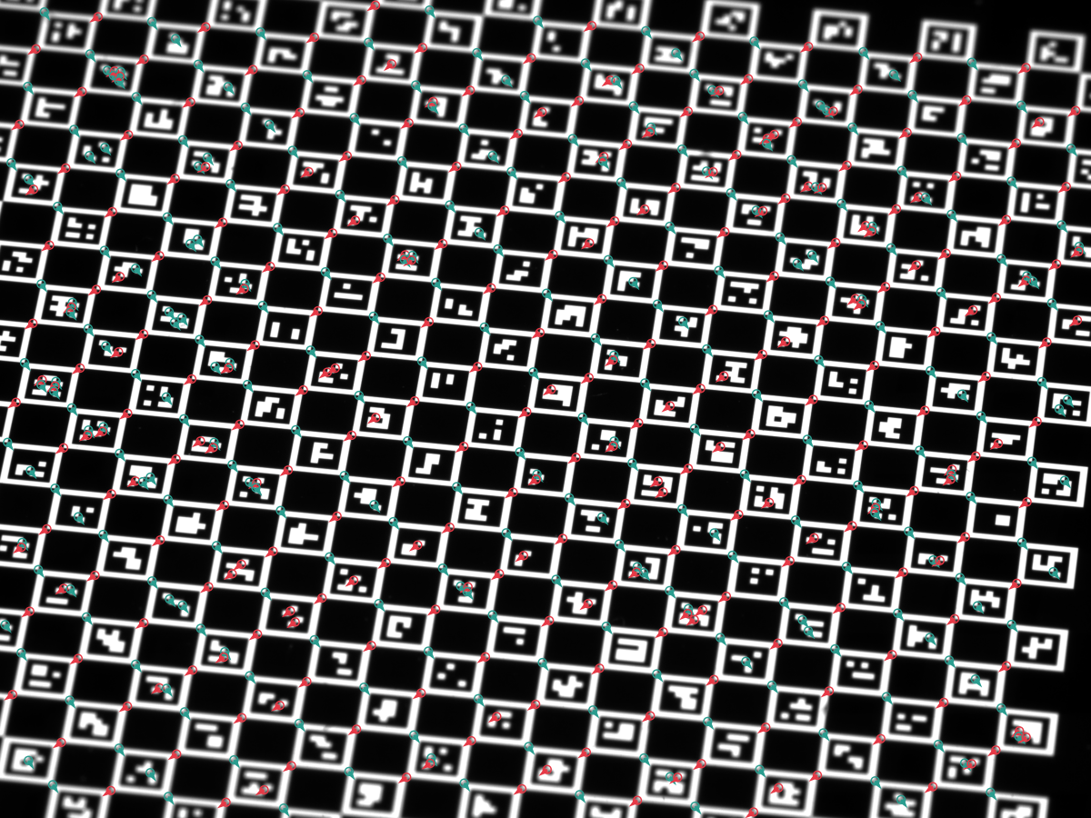
Overlay examples on the sample images in testdata/:
2.6 ML refiner
The ML refiner is a separate, optional code path. Enable it by
building with --features ml-refiner (Rust) or by installing a
wheel built with the same feature (Python), then pick the
Ml variant on the active ChESS refiner:
#![allow(unused)]
fn main() {
#[cfg(feature = "ml-refiner")]
{
use chess_corners::{ChessRefiner, Detector, DetectorConfig};

let cfg = DetectorConfig::chess_multiscale()
    .with_chess(|c| c.refiner = ChessRefiner::Ml);

let mut detector = Detector::new(cfg).unwrap();
let corners = detector.detect(&img).unwrap();
}
}
The ML path:
- Runs the ChESS detector to produce seeds.
- Feeds each seed’s 21×21 neighborhood through the embedded
ONNX model (
chess_refiner_v4.onnx, ~180 K params). - Replaces the seed position with the model’s predicted
(dx, dy)offset. - Falls back to the configured classical refiner if the ML path rejects or times out.
The algorithm and its limits are covered in Part V §5.6. The ML refiner is not a direct replacement for RadonPeak: in the Part VIII synthetic benchmark, RadonPeak has lower clean/blurred error and ML has lower mean error on the heaviest noise row.
The ML refiner lives on the ChESS strategy only — RadonRefiner does
not list an Ml variant.
2.7 Radon heatmap (visualization)
The Radon detector computes a dense (max_α S_α − min_α S_α)²
response heatmap as an intermediate step. The heatmap is exposed
across all wrappers for visualization, debugging, and downstream
tooling — useful when tuning ray_radius, image_upsample, or the
threshold floor.
The heatmap is returned at working resolution: the input is
optionally upscaled (DetectorConfig.upscale) and then internally
supersampled by the Radon detector (RadonConfig.image_upsample,
default 2). The working-to-input scale factor is therefore
upscale_factor * image_upsample. Multiply input-pixel coordinates by
this factor to land on heatmap pixels.
Rust:
#![allow(unused)]
fn main() {
use chess_corners::diagnostics::radon_heatmap_u8;
use chess_corners::DetectorConfig;

fn run(img: &[u8], width: u32, height: u32) {
let cfg = DetectorConfig::radon();
let map = radon_heatmap_u8(img, width, height, &cfg);
println!("heatmap {}×{}, max = {:.1}",
    map.width(), map.height(),
    map.data().iter().copied().fold(f32::NEG_INFINITY, f32::max));
}
}
Python:
import chess_corners
import numpy as np

cfg = chess_corners.DetectorConfig.radon()
detector = chess_corners.Detector(cfg)
heatmap = detector.radon_heatmap(img)  # (H', W') float32
print(heatmap.shape, heatmap.dtype, float(heatmap.max()))
WebAssembly (JS):
import init, { ChessDetector, DetectorConfig } from '@vitavision/chess-corners';

await init();
const det = ChessDetector.withConfig(DetectorConfig.radon());

const heatmap = det.diagnostics_radon_heatmap(grayPixels, width, height);
const w = det.diagnostics_radon_heatmap_width();
const h = det.diagnostics_radon_heatmap_height();
const scale = det.diagnostics_radon_heatmap_scale();  // working-to-input factor
console.log('heatmap', w, 'x', h, 'scale', scale);
The heatmap is independent from corner detection: calling it does not require the active strategy to be Radon, and it does not return corners.
In this part we focused on the public faces of the detector: the
image helper, the raw buffer API, the CLI, and the Python and JS
bindings. In the next parts we will look under the hood at how the
ChESS response is computed, how the detector turns responses into
subpixel corners, and how the multiscale pipeline is structured.
Next: Part III describes the ChESS response kernel, the detection pipeline, and the corner descriptor fit. Part IV covers the Radon detector.
Part III: The ChESS response detector
ChESS (Chess-board Extraction by Subtraction and Summation,
Bennett & Lasenby, 2014; CVIU
118:197–210) is a ring-based corner detector specialized
for chessboard X-junctions. Given an 8-bit grayscale image, it produces
a dense response map; positive values mark chessboard-like corners,
while edges, blobs, and flat regions should have lower response on the
ideal checkerboard model. The benchmark chapter reports single-digit
millisecond timings for the measured camera-sized test images with the
simd or rayon features enabled.
For a self-contained overview of the algorithm, see the chess-corners atlas page on vitavision.dev.
This part covers the ChESS pipeline end-to-end: the ring geometry, the response formula, the dense response computation over the image, the detection pipeline (threshold + NMS + cluster filter + subpixel refinement), and the corner descriptor that both detectors (ChESS here and Radon in Part IV) feed into.
The core ChESS code lives under
crates/chess-corners-core/src/detect/chess/ and the descriptor code
under crates/chess-corners-core/src/orientation/.
Feature flags (std, rayon, simd, tracing) only affect
performance and observability, not the numerical output.
3.1 Rings and sampling geometry
The ChESS response is built around a fixed 16‑sample ring at a
given radius. The core crate encodes these rings in
crates/chess-corners-core/src/ring.rs.
3.1.1 Canonical rings
The main types are:
RingOffsets– an enum representing the supported ring radii (R5andR10).RING5/RING10– the actual offset tables for radius 5 and 10.ring_offsets(radius: u32)– helper returning the offset table for a given radius (anything other than 10 maps to 5).
The 16 offsets are ordered clockwise starting at the top, and are derived from the FAST‑16 pattern:
RING5is the canonicalr = 5ring used in the original ChESS paper.RING10is a scaled variant (r = 10) with the same angles, which improves robustness under heavier blur at the cost of a larger footprint and border margin.
The exact offsets are stored as integer (dx, dy) pairs, so sampling
around a pixel (x, y) means accessing (x + dx, y + dy) for each
ring point.
3.1.2 From parameters to rings
ChessParams in lib.rs controls which ring to use:
use_radius10– whentrue,ring_radius()returns 10 instead of 5.descriptor_use_radius10– optional override specifically for the descriptor ring; whenNone, it followsuse_radius10.
Convenience methods:
ring_radius()/descriptor_ring_radius()return the numeric radii.ring()/descriptor_ring()returnRingOffsetsvalues, which can be turned into offset tables viaoffsets().
The response path uses ring(), while descriptor estimation uses
descriptor_ring(). This allows you, for example, to detect corners
with a smaller ring but compute descriptors on a larger one.
3.2 Dense response computation
The main entry point in response.rs is:
#![allow(unused)]
fn main() {
pub fn chess_response_u8(img: &[u8], w: usize, h: usize, params: &ChessParams) -> ResponseMap
}
This function computes the ChESS response at each pixel center whose full ring fits entirely inside the image. Pixels that cannot support a full ring (near the border) get response zero.
3.2.1 ChESS formula
For each pixel center c, we gather 16 ring samples s[0..16) using
the offsets described in §3.1, and a small 5‑pixel cross at the
center:
- center
c, - north/south/east/west neighbors.
From these values we compute:
-
SR– a “square” term that compares opposite quadrants on the ring:SR = sum_{k=0..3} | (s[k] + s[k+8]) - (s[k+4] + s[k+12]) | -
DR– a “difference” term encouraging edge‑like structure:DR = sum_{k=0..7} | s[k] - s[k+8] | -
μₙ– the mean of all 16 ring samples. -
μₗ– the local mean of the 5‑pixel cross.
The final ChESS response is:
R = SR - DR - 16 * |μₙ - μₗ|
Intuitively:
SRis large when opposite quadrants have contrasting intensities (as in an X‑junction).DRis large for simple edges, and subtracting it de‑emphasizes edge‑like structures.|μₙ - μₗ|penalizes isolated blobs or local illumination changes.
High positive values of R correspond to chessboard‑like corners.
3.2.2 Implementation paths and borders
chess_response_u8 is implemented in a few interchangeable ways:
- Scalar sequential path (
compute_response_sequential/compute_row_range_scalar) – a straightforward nested loop over rows and columns. - Parallel path (
compute_response_parallel) – when therayonfeature is enabled, the outer loop is split across threads usingpar_chunks_mutover rows. - SIMD path (
compute_row_range_simd) – when thesimdfeature is enabled, the inner loop vectorizes overLANESpixels at a time, using portable SIMD to gather ring samples and accumulateSR,DR, andμₙin vector registers.
Regardless of the path, the function:
- respects a border margin equal to the ring radius so that all ring accesses are in bounds,
- writes responses into a
ResponseMap { w, h, data }in row‑major order, - keeps the scalar, parallel, and SIMD variants within the documented deterministic-output contract.
3.2.3 ROI support with Roi
For multiscale refinement, we rarely need the response over the entire image. Instead we compute it inside small regions of interest around coarse corner predictions.
The Roi struct:
#![allow(unused)]
fn main() {
pub struct Roi {
    pub x0: usize,
    pub y0: usize,
    pub x1: usize,
    pub y1: usize,
}
}
describes an axis‑aligned rectangle in image coordinates. A specialized function:
#![allow(unused)]
fn main() {
pub fn chess_response_u8_patch(
    img: &[u8],
    w: usize,
    h: usize,
    params: &ChessParams,
    roi: Roi,
) -> ResponseMap
}
computes a response map only inside that ROI, treating the ROI as a small image with its own (0,0) origin. This is used in the multiscale pipeline to refine coarse corners without paying the cost of full‑frame response computation at the base resolution.
3.3 Detection pipeline
The response map is only the first half of the detector. The second
half—implemented in detect.rs—turns responses into subpixel corner
candidates.
3.3.1 Thresholding and NMS
The main stages are:
- Thresholding – we reject responses that are too small to be
meaningful. The paper’s contract is “any strictly positive
Ris a corner candidate”, which is what the default settings encode:- The default is
Threshold::Absolute(0.0)combined with a strictR > thrcomparison, i.e. accept iffR > 0. - Callers can opt into
Threshold::Relative(frac)(a fraction of the maximum response in the current frame) — useful as an adaptive policy on high‑contrast scenes where the raw positive‑response floor contains sensor noise. - Or tune the absolute threshold upward directly with
Threshold::Absolute(value)to suppress flat‑region noise without committing to a scene‑max policy.
- The default is
- Non‑maximum suppression (NMS) – in a window of radius
nms_radiusaround each pixel, we keep only local maxima and suppress weaker neighbors. - Cluster filtering – we require that each surviving corner have
at least
min_cluster_sizepositive‑response neighbors in its NMS window. This discards isolated noisy peaks that don’t belong to a structured corner.
The result of this stage is a set of raw corner candidates, each carrying:
- integer‑like peak position,
- response strength (before refinement).
3.3.2 Subpixel refinement
Each candidate is refined from its integer peak to a subpixel
position by one of the refiners in
Part V. The ChESS detector is selected via
DetectorConfig.refiner.kind; the default is CenterOfMass, which
operates directly on the response map, but any of the five refiners
can be used. Refinement is a per-candidate call and adds at most a
few tens of nanoseconds for the fastest options.
The internal type representing a refined candidate is
descriptor::Corner:
#![allow(unused)]
fn main() {
pub struct Corner {
    /// Subpixel location in image coordinates (x, y).
    pub xy: [f32; 2],
    /// Raw ChESS response at the integer peak (before refinement).
    pub strength: f32,
}
}
The refinement step preserves the detector’s noise robustness and adds subpixel precision. Measured accuracy and throughput for each refiner are in Part VIII.
3.4 Corner descriptors
Raw corners (position + strength) are enough for many applications,
but the core crate also offers a richer CornerDescriptor that fits
a parametric intensity model to the 16-sample ring around each corner.
The fit yields both local grid axes independently, their per-axis
1σ angular uncertainty, a bright/dark contrast amplitude, and the RMS
fit residual — all in one pass.
Both the ChESS detector and the Radon detector produce
CornerDescriptor values via the same describe_corners
function, so everything in this section applies to both pipelines.
3.4.1 CornerDescriptor
Defined in descriptor.rs:
#![allow(unused)]
fn main() {
pub struct CornerDescriptor {
    pub x: f32,
    pub y: f32,
    pub response: f32,
    pub contrast: f32,
    pub fit_rms: f32,
    pub axes: [AxisEstimate; 2],
}

pub struct AxisEstimate {
    pub angle: f32,
    pub sigma: f32,
}
}
Fields:
x,y– subpixel coordinates in full‑resolution image pixels.response– raw, unnormalized ChESS responseR = SR − DR − 16·MRat the detected peak. Units are 8‑bit pixel sums; the paper’s contract isR > 0.contrast– fitted bright/dark amplitude|A|in gray levels. Independent fromresponseand not comparable to it.fit_rms– root‑mean‑squared residual of the two‑axis intensity fit (gray levels). Smaller means the ring sampled cleanly through a chessboard‑like corner.axes[0],axes[1]– the two local grid axis directions and their 1σ uncertainties.
The axis convention:
axes[0].angle ∈ [0, π)— the “line direction” of axis 1.axes[1].angle ∈ (axes[0].angle, axes[0].angle + π).- Rotating CCW from
axes[0].angletowardaxes[1].angletraverses a dark sector; the second half‑turn crosses the other dark sector, and the remaining two sectors are bright. - The two axes are not assumed orthogonal — a projective warp (or strong lens distortion) tilts the two sectors independently.
3.4.2 Two‑axis intensity model
The ring samples s₀, …, s₁₅ at angles φ₀, …, φ₁₅ = atan2(dy, dx)
are fitted to
I(φ) = μ + A · tanh(β·sin(φ − θ₁)) · tanh(β·sin(φ − θ₂))
with fixed β = 4.0. The four free parameters are:
μ– ring‑level mean intensity,A– bright/dark amplitude (signed during optimization, canonicalized to non‑negative on exit),θ₁,θ₂– the two grid axis directions.
Intuition: each tanh(β · sin(φ − θᵢ)) is a smooth approximation of
sign(sin(φ − θᵢ)), i.e. +1 on one side of the axis line and −1 on
the other. Their product is +1 in two antipodal “bright” sectors and
−1 in the two “dark” sectors, matching a chessboard X‑junction. The
fixed β reflects the effective ring‑integration blur at the sampled
radius and is not a fit parameter.
3.4.3 Gauss–Newton solver
fit_two_axes runs a small Gauss–Newton iteration (up to 6 steps):
- Seed
θ₁,θ₂from the 2nd-harmonic Fourier coefficient of the centred ring samples, placed at the sector midpoint ± π/4. SeedAfrom the harmonic magnitude. The initial 90° spacing is only a seed — the two angles are independent free parameters during optimisation. - At each step, evaluate the residuals and the 16×4 Jacobian of
I(φᵢ)with respect to[μ, A, θ₁, θ₂]and solve the normal equationsJᵀJ · Δ = Jᵀ rwith partial pivoting. - Clamp angular updates to ±0.5 rad per step to prevent runaway.
- Stop once the update falls below
‖Δθ‖ < 10⁻⁴or the iteration cap is reached. - Canonicalize
(θ₁, θ₂, A)so thatA ≥ 0,θ₁ ∈ [0, π)and the CCW arc fromθ₁toθ₂spans a dark sector.
Flat or near‑flat rings (ring variance below 10⁻⁶, or 2nd‑harmonic
magnitude below 10⁻⁴) short‑circuit to a degenerate fit:
A = 0, θ₁ = 0, θ₂ = π/2, and σ = π on both axes so downstream
consumers can detect the “no signal” case via the uncertainty field.
3.4.4 Per‑axis 1σ uncertainty
The sigma field on each AxisEstimate is the standard 1σ angular
uncertainty from the linearised Gauss–Newton covariance at the
optimum:
- The sum of squared residuals is
SSR = Σᵢ (sᵢ − I(φᵢ))². - The unbiased residual variance is
σ̂² = SSR / (N − p) = SSR / (16 − 4) = SSR / 12. - The parameter covariance is
Σ = σ̂² · (JᵀJ)⁻¹, whereJᵀJis the final Gauss–Newton normal matrix. - The angle sigmas are the relevant diagonal entries:
σθ₁ = √Σ[2,2],σθ₂ = √Σ[3,3](clamped to ≥ 0, capped at π).
This is the textbook Cramér–Rao‑style uncertainty for nonlinear
least squares — it assumes residuals are approximately iid Gaussian
and the linearisation around the optimum is adequate. It does not
account for model mismatch (e.g. a corner that is not well described
by a separable two‑axis tanh product), but it scales correctly with
SNR: noisier rings produce proportionally larger sigma.
Practically, sigma is useful for:
- Weighting corners in downstream grid fitting (inverse‑variance weights, or rejecting corners whose axes are too uncertain).
- Flagging degenerate fits:
sigma ≈ πmeans the fit did not lock onto a well‑defined grid.
3.4.5 From corners to descriptors
The function:
#![allow(unused)]
fn main() {
pub fn describe_corners(
    img: &[u8],
    w: usize,
    h: usize,
    radius: u32,
    corners: Vec<Corner>,
    method: OrientationMethod,
) -> Vec<CornerDescriptor>
}
turns raw Corner values into full descriptors by:
- Sampling the 16‑point ring around each corner with bilinear
interpolation (
sample_ring). - Running
fit_two_axesto obtain(μ, A, θ₁, θ₂), the Gauss–Newton covariance, and the residual RMS. - Canonicalising the axes and packaging everything into a
CornerDescriptor.
The pass is deterministic and purely local — there is no global optimisation or topology reasoning at this stage.
3.4.6 When to use descriptors
You get CornerDescriptor values when you use the high‑level APIs:
chess-corners-coreusers can run the response and detector stages manually and then callchess_corners_core::describe_corners.chess-cornersusers getVec<CornerDescriptor>directly from theDetectorstruct’sdetect,detect_u8, ordetect_viewmethods.
For many tasks, x, y, and response are enough. When you need
more insight into local structure — grid fitting, lens‑distortion
modelling, calibration with per‑corner weights, or outlier rejection
before bundle adjustment — axes, sigma, contrast, and fit_rms
are the extra handles you get “for free” with each detection.
The axes, sigma_theta1, sigma_theta2, amp, and fit_rms
fields are produced by an orientation method shared with the Radon
detector. See Part VI: Orientation methods
for the API surface, the two available algorithms (RingFit and
DiskFit), and step-by-step descriptions of each.
Next: Part IV covers the alternative Radon response detector, which shares the descriptor pipeline above but uses a ray-based kernel instead of a ring.
Part IV: The Radon response detector
The ChESS detector of Part III samples a ring of 16 pixels around each candidate and computes a single response value per pixel. It assumes enough image support to fill the ring cleanly. Under strong blur, severe defocus, low contrast, or cell sizes smaller than about twice the ring radius, that support breaks down and the ring response stops being selective.
The Radon response detector is an alternative based on Duda & Frese (2018), “Accurate Detection and Localization of Checkerboard Corners for Calibration” (BMVC). Instead of a ring, it integrates along four rays through each candidate pixel and uses the gap between the strongest and weakest ray as the corner response. The computation is kept O(1) per pixel using summed-area tables.
For a self-contained overview of the algorithm, see the duda-radon-corners atlas page on vitavision.dev.
The Radon detector is a full alternative to ChESS — same input
(&[u8] grayscale), same output
(CornerDescriptor),
same place in the pipeline. It is selected via DetectorConfig.strategy
by setting it to DetectionStrategy::Radon(RadonConfig).
4.1 Ray response
For a candidate pixel (x, y) and a ray half-length r (working-resolution
pixels), we sum pixel intensities along four rays passing through the
pixel at angles α ∈ {0, π/4, π/2, 3π/4}:
S_α(x, y) = Σ_{k=-r}^{r} I(x + k·cos α, y + k·sin α)
The four sums S₀, S_{π/4}, S_{π/2}, S_{3π/4} sample two pairs of
orthogonal directions (horizontal/vertical and the two diagonals). At
an X‑junction, two of the four rays lie near the dark/bright axes and
average toward opposite extremes; the other two cross the junction and
average toward the scene mean. The Radon response is the squared
gap between the largest and smallest ray sum:
R(x, y) = (max_α S_α − min_α S_α)²
R is always non-negative. On the idealized checkerboard model used
by the tests, it peaks at X-junctions and stays small on flat regions,
straight edges, and blobs because in each of those cases all four ray
sums end up close to each other.
The squaring keeps the response proportional to the square of image
contrast, which is the natural scale for a log-fit later. It also
removes the sign ambiguity between dark / bright and bright / dark
corner polarities.
4.2 O(1) ray sums via summed-area tables
Naively, each ray sum costs 2r + 1 pixel reads. Computing the full
response map at every pixel is then O(r · W · H), which scales with
the ray length. Four summed-area tables (SATs) reduce it to O(W · H),
independent of r:
| Table | Definition | Reads for S_α |
|---|---|---|
row_cumsum | T[y][x] = Σ_{k=0..x} I[y][k] | S_0 (horizontal ray) |
col_cumsum | T[y][x] = Σ_{k=0..y} I[k][x] | S_{π/2} (vertical) |
diag_pos_cumsum | T[y][x] = T[y-1][x-1] + I[y][x] (NW-SE) | S_{π/4} (main diag) |
diag_neg_cumsum | T[y][x] = T[y-1][x+1] + I[y][x] (NE-SW) | S_{3π/4} (anti-diag) |
Each SAT is built in one pass over the image. A ray sum then costs two
table lookups: S = T[end] − T[one past start]. The construction
logic and the lookup pattern are in the Radon response source inside
chess-corners-core (see chess_corners_core::unstable for the
sub-stage entry points exposed without semver guarantees).
SAT element type
The default SAT element is i64, which handles any image size up to
host memory. The radon-sat-u32 crate feature switches to u32,
which halves SAT memory and widens SIMD-friendly lanes. The tradeoff
is a safe-input cap of 255 · W · H ≤ u32::MAX, about 16 megapixels.
The entry point rejects inputs beyond that cap rather than letting
the SAT wrap silently.
4.3 Working resolution and image upsampling
The paper samples the image on a 2× supersampled grid to place ray
endpoints on half-pixel centers. RadonDetectorParams.image_upsample
controls this:
image_upsample = 1— detector operates on the input grid.image_upsample = 2— input is bilinearly upsampled 2× before SATs are built; all subsequent steps run at the higher resolution. This is the paper default and the facade preset value.
Higher factors are clamped to 2 (chess_corners_core::unstable::MAX_IMAGE_UPSAMPLE). The response
map and detected peaks live at working resolution; the detector
divides peak coordinates by image_upsample before returning them,
so output coordinates are always in the input pixel frame.
At image_upsample = 2, a ray_radius of 4 working-resolution
pixels covers 2 physical input pixels, which is the length used in
the paper’s benchmarks.
4.4 Peak fit pipeline
Once the dense response R(x, y) has been computed, the detector
turns it into subpixel corner positions with the same pipeline used
by the Radon refiner (see Part V):
- Box blur. A separable
(2·blur_radius + 1)²box filter smooths the response map in place.blur_radius = 1(a 3×3 box) is the facade preset and matches the paper-style peak-fit pipeline. - Threshold. Pixels below
threshold_abs(if set) orthreshold_rel · max(R)are dropped. BecauseR ≥ 0everywhere, there is no useful “strictly positive” selection analogous to ChESS’sR > 0; callers must pick a non-zero floor. Default isthreshold_rel = 0.01(1% of the map maximum). - Non-maximum suppression. Each surviving pixel must be the
strict maximum within a
(2·nms_radius + 1)²window. - Cluster filter. The pixel must have at least
min_cluster_sizepositive neighbors in the NMS window. Rejects isolated noise. - 3-point peak fit. Given the NMS winner
R_cat(x, y)and its four axial neighborsR_{x±1},R_{y±1}, fit a 1D parabola along each axis to find the subpixel offset. The paper’s Gaussian peak fit (PeakFitMode::Gaussian) fits the parabola tolog Rinstead, which is the MLE under the assumption that the peak is locally Gaussian. The parabolic fallback (PeakFitMode::Parabolic) operates on the rawRvalues.
The peak fit is a closed-form operation on three samples per axis —
no iteration. Implementation: radon::fit_peak_frac in
chess-corners-core.
Why these defaults
| Parameter | Default | Reason |
|---|---|---|
ray_radius | 4 | Paper value at image_upsample = 2; 2 physical pixels of support. |
image_upsample | 2 | Paper default. Halves aliasing on the ray endpoints. |
response_blur_radius | 1 | 3×3 box used by the preset and by the repository’s Radon tests. |
threshold_rel | 0.01 | 1 % of max(R). R ≥ 0 means a strictly positive threshold is required; 0.01 is a conservative floor. |
nms_radius | 4 | Matches ray_radius — local maxima should be at least one ray length apart. |
min_cluster_size | 2 | Requires at least one supporting positive neighbor inside the NMS window. |
peak_fit | Gaussian | Log-space 3-point fit used by the paper-style pipeline; parabolic fit is also available. |
4.5 When to pick ChESS vs Radon
Both detectors run on the same input and produce CornerDescriptor
values. The practical differences:
| Property | ChESS (Part III) | Radon (this chapter) |
|---|---|---|
| Support required | 16 samples at radius 5 or 10 | 4 rays of length 2·ray_radius + 1 |
| Minimum cell size in repo sweep | Degrades when the ring crosses neighbouring cells | Tested down to ~4 px with image_upsample = 2 |
| Gaussian blur in repo sweep | Degrades near σ ≈ 1.5 px | Lower error through σ ≈ 2.5 px on that fixture |
| Defocus / blur mechanism | Ring samples can smear across cells | Ray integral averages over a short support |
| Cost per image | One ring sample per pixel (+SIMD) | 4 SATs + one dense map per pixel |
| Memory overhead | One ResponseMap | Four SATs + response + blur scratch |
| Subpixel refinement | Needs a separate refiner stage | Built into the detector’s peak fit |
ChESS is faster on the measured clean test images. The Radon detector is useful when the ChESS ring response does not seed enough corners, especially in the synthetic small-cell, blur, and low-contrast cases covered by the tests and Part VIII. Treat those measurements as guidance and validate on your own image distribution when the tradeoff matters.
The two detectors are not meant to be stacked. They are peers, and
the DetectorConfig.strategy enum picks one.
4.6 Public API
Core crate
chess_corners_core exposes the Radon pipeline at two levels.
Low-level — response map only:
#![allow(unused)]
fn main() {
use chess_corners_core::{
RadonBuffers, RadonDetectorParams, radon_response_u8,
};
let mut buffers = RadonBuffers::new();
let params = RadonDetectorParams::default();
let resp = radon_response_u8(&img_u8, width, height, ¶ms, &mut buffers);
println!("response map is {}×{}", resp.width(), resp.height());
}RadonBuffers holds the upsampled image, the four SATs, the response
map, and the blur scratch. Construct it once and reuse across frames
to avoid per-frame allocations.
Full pipeline — detect corners:
#![allow(unused)]
fn main() {
use chess_corners_core::{
detect_peaks_from_radon, radon_response_u8, RadonBuffers, RadonDetectorParams,
};
let mut buffers = RadonBuffers::new();
let params = RadonDetectorParams::default();
let resp = radon_response_u8(&img_u8, width, height, ¶ms, &mut buffers);
let corners = detect_peaks_from_radon(&resp, ¶ms);
// corners: Vec<Corner> — each has (x, y, strength) in input pixels.
}Facade crate
DetectorConfig::radon() is a preset that selects the Radon detector
and all its defaults:
#![allow(unused)]
fn main() {
use chess_corners::{DetectorConfig, Detector};

let cfg = DetectorConfig::radon();      // strategy = Radon(RadonConfig)
let mut detector = Detector::new(cfg)?;
let corners = detector.detect(&gray_image)?;
// corners: Vec<CornerDescriptor>
}
The facade runs the Radon detector, feeds its output into
describe_corners (the shared descriptor stage from Part III §3.4),
and returns CornerDescriptor values in the input pixel frame. The
orientation method that fills axes and sigma_theta* is shared with
the ChESS pipeline; see Part VI: Orientation methods.
4.7 Coarse-to-fine Radon
DetectorConfig::radon_multiscale() enables the same coarse-to-fine
2× pyramid that the ChESS pipeline uses (see
Part VII), driven by the Radon
response kernel. The multiscale field is top-level on DetectorConfig
and is honoured by both detectors symmetrically:
#![allow(unused)]
fn main() {
use chess_corners::{DetectorConfig, Detector, MultiscaleConfig};

// Three-level coarse-to-fine Radon preset:
let cfg = DetectorConfig::radon_multiscale();

// Tune a nested Radon field via the closure mutator:
let cfg = DetectorConfig::radon_multiscale()
    .with_radon(|r| r.ray_radius = 6);

// Or set the pyramid depth directly:
let mut cfg = DetectorConfig::radon_multiscale();
cfg.multiscale = MultiscaleConfig::pyramid(2, 128, 3);

let mut detector = Detector::new(cfg)?;
let corners = detector.detect(&gray_image)?;
}
When to try radon_multiscale before single-scale radon:
- Large frames (≥ 1280 × 960) where full-resolution Radon response cost dominates the frame budget.
- Blurry or low-contrast imagery across a large field of view where the ChESS preset does not emit enough seeds.
- Tight latency budgets on large sensors where single-scale
radonis too slow and the ChESS multiscale preset misses corners.
For small frames or when per-frame latency is not a concern,
single-scale radon is simpler and worth measuring against the
multiscale preset.
Tuning
The active [RadonConfig] inside
DetectionStrategy::Radon exposes
every field in §4.4’s defaults table. The most common tweaks:
- Heavy blur or low contrast: try
ray_radiusin the 5–6 working-pixel range. - Small cells (3–4 physical pixels): keep
image_upsample = 2; reduceray_radiusto 2–3. - Very clean data: try
response_blur_radius = 0and a higher relative threshold (for example 0.05) to cut weak peaks. - Noise-heavy scenes: try
response_blur_radius = 2and verify the result count and residuals.
Next we move from response maps to what happens after detection: Part V describes the subpixel refiners that can replace the Radon peak-fit when the ChESS detector is in use, and that can also refine Radon output when extra precision is needed.
Part V: Subpixel refiners
A corner detector (ChESS or Radon) returns integer pixel positions
plus a response value. Most downstream consumers — camera calibration,
pose estimation, homography fitting — need positions to better than a
pixel. A refiner takes one seed (x₀, y₀) plus a local view into
either the image or the response map and returns a refined
(x, y) in subpixel coordinates.
The library ships five refiners with one trait and one configuration enum, so swapping between them is a one-line change. The ChESS detector always runs one of these refiners to reach subpixel accuracy. The Radon detector has its own peak fit built in (see Part IV §4.4), but its output can still be post-refined if you need a different statistical behavior.
5.1 The refiner trait
#![allow(unused)]
fn main() {
pub trait CornerRefiner {
    /// Half-width of the patch the refiner reads around the seed.
    fn radius(&self) -> i32;

    /// Refine one seed. `ctx` exposes the image and/or response map.
    fn refine(&mut self, seed_xy: [f32; 2], ctx: RefineContext<'_>) -> RefineResult;
}
}
A RefineResult carries the refined (x, y), a refiner-specific
score, and a RefineStatus:
Accepted— refined position is insideradius-sized support and below the refiner’s rejection thresholds.OutOfBounds— the patch would read past the image border.IllConditioned— the refiner’s local system was singular or too eccentric (edge rather than corner).Rejected— the refined offset exceeded the refiner’smax_offset, or a per-refiner score threshold fired.
The user-facing selector is per-detector: ChessRefiner (carrying
CenterOfMass, Forstner, SaddlePoint, and optionally Ml) lives
inside ChessConfig; RadonRefiner (carrying RadonPeak and
CenterOfMass) lives inside RadonConfig. Each enum variant carries
its tuning struct as a payload, so a refiner kind change cannot leave
a stale per-refiner config field behind. At runtime the facade stores
an owned Refiner enum (one allocated scratch buffer per concrete
refiner) so the same instance is reused across seeds — no per-corner
allocation.
5.2 CenterOfMass
Operates on the ChESS response map. Computes the response-weighted
centroid of a (2r + 1)² window around the seed:
x_r = Σ_{p in W}  (x_p · R_p)  /  Σ_p R_p
y_r = Σ_{p in W}  (y_p · R_p)  /  Σ_p R_p
R_p = max(R(x, y), 0) clips negative responses so one strong
negative pixel can’t push the centroid outside the window.
| Property | Value |
|---|---|
| Input | Response map |
Default radius | 2 (5×5 window) |
| Typical cost | ~20 ns per corner |
| Strengths | Cheapest option in the benchmark; closed-form |
| Weaknesses | Centroid bias when the response is asymmetric; |
fails when radius crosses neighboring corners |
Use when throughput matters more than sub-0.1 px accuracy, or when the ChESS response is the only signal you want the refinement to see.
5.3 Förstner
Gradient-based. Solves a weighted least-squares system for the point closest (in a Mahalanobis sense) to all image-gradient lines in a local window. The structure tensor
M = Σ_p  w_p · [ gx²  gx·gy ]
               [ gx·gy  gy²  ]
is assembled with 3×3 central-difference gradients and radial
weights w_p = 1 / (1 + 0.5·‖p − seed‖²). The refined position is
u = M⁻¹ · Σ_p w_p · (p − seed) · [gx·gy]ᵀ
Rejections:
trace(M) < min_trace— low-gradient region.det(M) < min_det— singular structure tensor.λ_max / λ_min > max_condition_number— one dominant direction (an edge, not a corner).‖u‖ > max_offset— extrapolating beyond a trusted neighborhood.
| Property | Value |
|---|---|
| Input | Image |
Default radius | 2 (5×5 gradient window + 1 px halo) |
| Typical cost | ~60 ns per corner |
| Strengths | Principled on sharp, high-SNR images |
| Weaknesses | Relies on sharp gradients — blur flattens M |
Good pick for clean calibration frames where image edges are sharp. In the synthetic blur sweep in Part VIII, Gaussian blur flattens the gradient magnitudes and this refiner’s error increases with σ.
Reference: Förstner & Gülch, 1987, “A fast operator for detection and precise location of distinct points, corners and centres of circular features.”
5.4 SaddlePoint
Fits a 2D quadratic f(x, y) = a·x² + b·x·y + c·y² + d·x + e·y + g
to a (2r + 1)² image patch and returns the saddle point (the
critical point where ∇f = 0). The six coefficients come from a
6×6 normal-equation solve with partial pivoting.
The determinant of the Hessian is 4·a·c − b². A true X‑junction is a
saddle, so the Hessian should be indefinite (det < 0). The refiner
rejects:
|det| < min_abs_det— flat patch.det > -det_margin— the quadratic is a bowl or ridge, not a saddle.‖offset‖ > max_offset— refined point outside the patch.
| Property | Value |
|---|---|
| Input | Image |
Default radius | 2 (5×5 patch) |
| Typical cost | ~120 ns per corner |
| Strengths | No gradient required; low error in the blur sweep |
| Weaknesses | Parabolic model is approximate on sharp edges |
A reasonable default when you do not know in advance whether frames will be sharp or blurred. In Part VIII’s synthetic blur sweep it stays inside the same error band as the other non-Förstner geometric refiners.
5.5 RadonPeak
Per-candidate version of the Radon detector’s peak fit. Computes the
local Radon response on a (2·patch_radius + 1)² grid around the
seed (at working resolution set by image_upsample), applies the
same 3×3 box blur and 3-point Gaussian peak fit used by the full
detector, and returns the refined offset. See
Part IV §4.4 for
the underlying formulas — this refiner shares all of them.
| Property | Value |
|---|---|
| Input | Image |
| Default settings | ray_radius = 2, patch_radius = 3, image_upsample = 2 |
| Typical cost | ~17 µs per corner |
| Strengths | Lowest clean/blurred error in the benchmark |
| Weaknesses | 100–1000× slower than the structure-tensor refiners |
This is the lowest-error option on the clean and blurred synthetic rows reported in Part VIII. Choose it when that extra accuracy matters more than the added per-corner cost.
If you are already running the Radon detector (Part IV), its built-in peak fit gives you the same refinement implicitly, and this refiner is redundant.
5.6 ML (ONNX model)
A learned refiner. Feeds a 21×21 normalized grayscale patch into a
small CNN and takes [dx, dy, conf_logit] back out. The ChESS path
extracts the patch, stages a batch, runs ONNX inference via
tract-onnx, and adds [dx, dy] to each seed.
Available behind the ml-refiner feature. The default model
chess_refiner_v4.onnx is embedded in the
chess-corners-ml crate at
crates/chess-corners-ml/assets/ml/.
5.6.1 Architecture
The shipped model is CornerRefinerNet, a CoordConv CNN with a
flatten + MLP head. About 180 K parameters:
| Layer | Shape | Notes |
|---|---|---|
| Input | 1 × 21 × 21 | Grayscale patch, normalized u8/255. |
| CoordConv prepend | 3 × 21 × 21 | Two extra channels with per-pixel x, y in [-1, 1]. |
| Conv3×3, ReLU | 16 × 21 × 21 | |
| Conv3×3, ReLU | 16 × 21 × 21 | |
| Conv3×3 stride 2, ReLU | 32 × 11 × 11 | |
| Conv3×3, ReLU | 32 × 11 × 11 | |
| Conv3×3 stride 2, ReLU | 64 × 6 × 6 | |
| Flatten | 2304 | |
| Linear, ReLU | 64 | |
| Linear (no activation) | 3 | [dx, dy, conf_logit]. |
CoordConv (Liu et al., 2018) concatenates explicit x, y coordinate
channels to the input. Standard convolutions are translation-equivariant
and cannot reliably regress to an absolute pixel offset from a patch
center; CoordConv restores the center reference that pure convolutions
discard.
The head outputs three scalars: an offset (dx, dy) in patch-pixel
units (valid range about [-0.6, 0.6] px, matching the training
distribution) and a confidence logit. The current Rust consumer
applies the offset and ignores the confidence.
The PyTorch source in tools/ml_refiner/model.py also defines a
wider variant (CornerRefinerNetLarge, ~730 K params, GroupNorm
between convs) and a spatial-softargmax head
(CornerRefinerNetSoftArgmax). Both match the 1-channel in, 3-scalar
out contract so they are drop-in replacements for the inference
path. The shipped model is the small variant — the larger and
softargmax variants did not move the held-out error meaningfully in
our sweeps.
5.6.2 Training data and loss
The training pipeline lives in tools/ml_refiner/. The v4 dataset
(configs/synth_v6.yaml) renders 200 000 patches with a 50/50 mix of
two rendering modes:
- Hard cells. An anti-aliased periodic checkerboard, rendered at
a random cell size in
[4, 12]px, then blurred by a Gaussian PSF inσ ∈ [0.3, 2.0]px. This matches real camera output: ink/paper step edges, softened by the optical system’s PSF, sampled by the sensor. The benchmark fixture in Part VIII uses the same renderer. - Smooth saddle. The
tanh(x)·tanh(y)model from earlier dataset revisions. Included at 50 % weight so callers who still feed the model smooth synthetic patches — as older documentation suggested — keep working.
Augmentations per sample: additive Gaussian noise σ ∈ [0, 10] gray
levels, photometric jitter (contrast, brightness, gamma), optional
projective warp for perspective robustness, and 20 % negative
samples (flat, edge, stripe, blob, pure noise, near-corner) with
is_pos = 0.
The true subpixel offset is sampled from [-0.6, 0.6] px.
Loss: Huber on (dx, dy) for positives, binary cross-entropy on
confidence for all samples. The regression loss is weighted up on
positives only via is_pos (negatives have no valid target).
5.6.3 Why earlier versions failed
Historical context, for anyone wondering why v4 is the version that
ships. Versions v1–v2 trained exclusively on smooth tanh(x)·tanh(y)
corner patches. That patch model does not resemble what a camera
produces — real sensor images have hard step edges (ink/paper)
softened by a small optical PSF, whereas tanh has smooth transitions
the width of the entire patch. Models trained on tanh only generalized
poorly to the benchmark fixture (mean error ~0.5 px on hard cells).
v3 swapped to hard cells only and hit ~0.6 px on tanh inputs — the
opposite distribution failure.
v4 is the mixed dataset (50/50) plus retuned offsets and augmentations.
In the Part VIII synthetic benchmark it avoids the earlier tanh /
hard-cell mismatch and has the lowest mean error on the heaviest noise
row (σ = 10 gray levels). It does not beat RadonPeak on clean or
mildly blurred data. The current evidence is that the training setup did
not learn the hand-designed RadonPeak structure; neither a wider CNN nor
a softargmax head closed that gap in the sweeps.
5.6.4 ONNX export and inference
The export step (tools/ml_refiner/export_onnx.py) writes an ONNX
graph at opset 17 (falling back to 18 if a conversion is unsupported).
The graph contract is:
- Input
patches:float32 [N, 1, 21, 21],u8 / 255in[0, 1]. - Output
pred:float32 [N, 3]with[dx, dy, conf_logit].
Rust inference is chess_corners_ml::MlModel::infer_batch. It wraps
tract-onnx, sizes the input to the runtime batch, and returns
Vec<[f32; 3]>. Dynamic batch sizing is supported via a tract
SymbolScope, so a single loaded model can handle variable-batch
calls without re-optimization.
5.7 Picking a refiner
The measurement-driven comparison lives in Part VIII. In short:
- Budget matters more than anything else: the structure-tensor refiners are 100–1000× faster than RadonPeak and ML.
- RadonPeak gives the lowest error on the clean and blurred synthetic rows, at a much higher per-corner cost.
- ML has the lowest mean error on the heaviest synthetic noise row.
- SaddlePoint is a conservative default when you want image-patch refinement without the cost of RadonPeak or ML.
The refiner is selected through the strategy’s refiner field.
For ChESS: DetectorConfig::chess().with_chess(|c| c.refiner = ChessRefiner::forstner()).
For Radon: DetectorConfig::radon().with_radon(|r| r.refiner = RadonRefiner::radon_peak()).
Switching is a single-line change, and the comparison numbers
in Part VIII come from running all five on the same fixture at a
single build.
Next, Part VI covers the orientation
methods that produce the axes and sigma_theta* descriptor fields,
shared by both the ChESS and Radon pipelines.
Part VI: Orientation methods
Both the ChESS detector and the Radon detector produce a list of corner candidates with subpixel positions. The descriptor pipeline lifts each position to a richer record that includes two grid-axis directions, their per-axis 1σ uncertainties, the corner contrast, and a fit residual. The “orientation method” is the algorithm that fits those axes from local image evidence — and because both detectors feed the same descriptor pipeline, the orientation method is detector-agnostic.
This chapter covers the two methods exposed by the public API, when to use each, and how each one works step by step.
6.1 API surface
The orientation_method field on DetectorConfig (and the
OrientationMethod enum) selects which algorithm runs:
| Method | JSON key | Notes |
|---|---|---|
RingFit | "ring_fit" | Default. 16-sample ring Gauss-Newton fit with calibrated σ. |
DiskFit | "disk_fit" | Full-disk crossing-line estimator. Falls back to RingFit on weak evidence. |
Both methods produce the same AxisFitResult shape:
(theta1, theta2, sigma_theta1, sigma_theta2, amp, rms). They differ
in the image evidence they use and in the failure modes they handle.
6.2 RingFit
RingFit samples 16 pixel values on a ring of radius \(r\) around the
corner center and fits the parametric two-axis chessboard intensity
model
\[ I(\varphi) = \mu + A \cdot \tanh\bigl(\beta \sin(\varphi - \theta_1)\bigr) \cdot \tanh\bigl(\beta \sin(\varphi - \theta_2)\bigr) \]
via Gauss-Newton, seeded from the 2nd-harmonic orientation of the ring samples. The slope \(\beta\) is fixed; the four free parameters are \(\mu, A, \theta_1, \theta_2\). Per-axis 1σ uncertainties are calibrated by a piecewise-linear LUT keyed on the contrast-relative residual, bringing reported sigmas closer to the empirical RMSE.
RingFit is suitable for the full range of standard chessboard images.
It is the default and should be left in place unless you have a
specific reason to switch.
6.3 When the ring fit isn’t enough
Three synthetic-patch cases motivate DiskFit and explain the
lazy-gate logic. In each figure, ground truth is dashed white, the
ring fit is red, and the disk fit is green.
Clean orthogonal corner
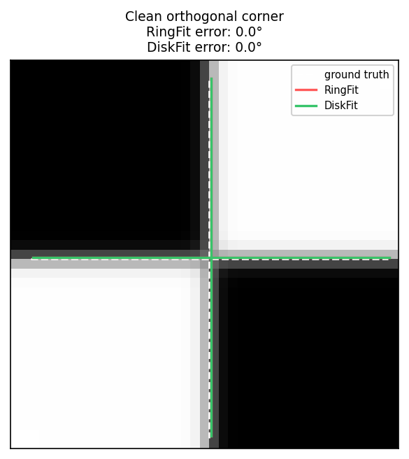
The 16-sample ring sits squarely on the four sectors of a canonical chessboard crossing. Both methods recover the axes within ~0.1°. The disk fit’s lazy gate detects this case from the ring’s contrast-relative residual (\(\text{rel_rms} < 0.04\)) and short-circuits to the ring fit, so you pay no extra cost on the easy corners.
Narrow projective skew
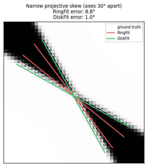
When projective warp pulls the two axes close together (here only 30° between them), the ring loses discriminative power: most ring samples sit in the two wide sectors and only a few sit in the narrow band between the lines. The 2nd-harmonic seed pulls the ring fit toward near-orthogonal axes, so it spreads the recovered angles outward (8.8° error). The disk fit looks at every pixel in the support disk — including the narrow-sector evidence the ring barely touches — and recovers both axes within 1°.
Sharp transition
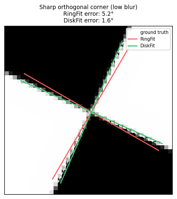
The ring fit’s parametric model fixes the tanh slope \(\beta = 4\), which matches a moderate edge width. On a sharp transition (\(w = 0.35\) px) the model cannot make its predicted intensity drop fast enough at the edge: the residual inflates and the angle estimate biases (5.2° error). The disk fit sweeps four widths \({0.35, 0.70, 1.40, 2.80}\) px and picks the one that minimises the relative residual, recovering both axes within 1.6°.
6.4 DiskFit, step by step
DiskFit models a corner as two crossing transition lines through the
detected center. The intensity at every pixel \(p\) in a support disk
around the center is fitted to
\[ I(p) = \mu + A \cdot \tanh!\Bigl(\frac{d_0(p)}{w}\Bigr) \cdot \tanh!\Bigl(\frac{d_1(p)}{w}\Bigr) \]
where \(d_0(p), d_1(p)\) are the signed perpendicular distances from \(p\) to the two lines and \(w\) is a discrete edge width drawn from \({0.35, 0.70, 1.40, 2.80}\) px. Recovering the corner means picking the line pair \((\theta_0, \theta_1)\) and width \(w\) that best reconstruct the disk’s pixel intensities.
The pipeline runs in seven steps:
-
Lazy-disk gate. If the ring fit’s relative residual
rms / max(amp, 1)is below0.04and its axes are near-orthogonal (separation in[70°, 110°]), return the ring fit unchanged. Most chessboard corners pass this gate. The expensive disk pipeline only runs on suspect corners — extreme skew, blur, or low contrast — that fail one of these conditions. -
Disk extraction. Sample a support disk of radius
1.6·r(capped at 8 px) around(cx, cy). Exclude the inner 1 px and any pixels outside the image. Require ≥ 64 valid pixels. For each pixel store its signed offset from the center, intensity, and 3×3 Sobel gradient (magnitude and direction). -
Candidate generation. Build up to 64 candidate line directions from three sources, dropping any new candidate within 1°–4° of an existing one:
- up to 8 peaks of a 72-bin gradient-direction histogram (smoothed
with
[0.25, 0.5, 0.25], pruned at 12% of the dominant peak); - both ring-fit seed angles ±
{0°, 4°, 8°}; - a coarse 30°-spaced global grid as a deterministic safety net.
Histogram peaks find the truly observable lines; seed offsets cover the easy case; the global grid catches degenerate gradient distributions.
- up to 8 peaks of a 72-bin gradient-direction histogram (smoothed
with
-
Pair pruning. Form all candidate pairs whose angular separation lies in
[12°, 89.5°]. Score each pair by Gaussian-weighted per-pixel gradient alignment (σ = 4°around each candidate angle). Keep the top 24 by score; force-include the pair closest to the ring-fit seed and the pair of the two strongest single-candidate alignments so high-evidence seeds are never dropped. -
Closed-form fit per pair × width. For each surviving pair and each width, compute
q_p = tanh(d₀_p/w) · tanh(d₁_p/w)for every disk pixel and solve the OLS regressionI_p − μ̂ ≈ A · q_pfor amplitudeAdirectly from sufficient statistics. The residualSSRfalls out of the same statistics — no second pass over the disk. The objective isrel_rms − 1.25·edge_score, with \( \text{rel_rms} = \mathrm{rms} / \max(|A|, 1) \). Keep the top 2 fits by deterministic comparator (objective, thenrel_rms, thenedge_score, then narrowerw, then smaller angles). -
Local refinement. Around each top-2 seed, grid-search angle perturbations at step sizes
{1°, 0.5°, 0.25°}(3×3 grid per step, 24 trials per seed). Width is held fixed. -
Acceptance. Replace the ring fit only when the disk fit clears minimum amplitude (
A ≥ 10), correlation (≥ 0.74), and edge support (≥ 0.035), AND one of:rel_rmsbeats the ring fit by absolute margin (≥ 0.03) or ratio (≤ 92%);- axis separation is strongly non-orthogonal (
< 55°); - axis separation is
≥ 75°ANDw ≤ 0.7px (sharp orthogonal); - the disk axes disagree with the ring axes by
> 12°and edge support is≥ 0.18.
When accepted, the per-axis sigma is recomputed from the recovered separation and
rel_rms(a 1.5°/3° floor depending on whether separation is≥ 55°or not, plus8·rel_rmscapped at 6°, all scaled by 0.55). When rejected but the disk and ring axes disagreed by more than 12°, the ring fit’s sigma is inflated to at least 10° to flag the ambiguity.
6.5 Choosing a method
DiskFit costs more per corner than RingFit in the orientation
benchmark (~131 µs vs ~15 µs for the measured case), but the lazy gate
short-circuits clean orthogonal inputs. Switch to DiskFit when working
with images that have known projective warp; otherwise leave the
default in place.
For the per-method precision/cost trade-off on the synthetic bench,
see the orientation bench REPORT.md in tools/orientation_bench/.
The patch overlays in §6.3 are reproducible via
tools/render_orientation_overlays.py.
Next: Part VII covers the multiscale pipeline that drives the detector across a Gaussian pyramid.
Part VII: Multiscale pipeline
Parts II–V treated detection mostly as a single-scale operation: one
call, one image, one response map. In practice, frames vary in scale
and blur — a chessboard can occupy a small fraction of a large sensor,
or sit far enough from the camera that the corner pattern is heavily
blurred. For those cases the chess-corners crate offers a
coarse-to-fine multiscale detector built on top of fixed 2× image
pyramids.
This part describes:
- the
DenseDetectortrait that abstracts over the two detectors, - how the pyramid utilities work,
- how the coarse-to-fine detector uses them,
- how to pick a multiscale configuration.
The multiscale path is available for both the ChESS and Radon
detectors. The multiscale: MultiscaleConfig field sits at the top
level of DetectorConfig and is honoured symmetrically by both.
MultiscaleConfig::SingleScale skips the pyramid entirely;
MultiscaleConfig::Pyramid { levels, min_size, refinement_radius }
enables it. See
Part IV §4.7 for
the Radon-specific preset and when to prefer it over single-scale
Radon.
7.0 The DenseDetector trait
The multiscale orchestrator in crates/chess-corners/src/multiscale.rs
is generic over a DenseDetector implementor. Two zero-sized marker
types in chess-corners-core satisfy the trait:
ChessDetector— drives the ChESS ring-based response.RadonDetector— drives the whole-image Duda-Frese Radon response.
#![allow(unused)]
fn main() {
// chess-corners-core public API (simplified)
pub trait DenseDetector {
    type Params;
    type Buffers: Default;
    type Response<'a> where Self: 'a, Self::Buffers: 'a;

    fn compute_response<'a>(
        &self,
        view: ImageView<'_>,
        params: &Self::Params,
        buffers: &'a mut Self::Buffers,
    ) -> Self::Response<'a>;

    fn detect_corners(
        &self,
        response: &Self::Response<'_>,
        params: &Self::Params,
        refine_border: i32,
    ) -> Vec<Corner>;

    fn compute_response_patch<'a>(
        &self,
        base: ImageView<'_>,
        roi: (usize, usize, usize, usize),
        params: &Self::Params,
        buffers: &'a mut Self::Buffers,
    ) -> Self::Response<'a>;
}
}
DenseDetector and its two implementors are public re-exports of
chess-corners-core, so the trait is available to downstream crates
that want to extend the pipeline with a custom response kernel.
Subpixel image-domain refinement (Förstner, saddle-point, …) is
not part of the trait — it runs detector-agnostically via
chess_corners_core::refine_corners_on_image.
The chess-corners facade routes the active DetectorConfig::strategy
variant to the corresponding DenseDetector implementor at the start of
each detect call; neither the user nor the multiscale code needs to
branch on the strategy explicitly.
7.1 Image pyramids
The pyramid builder itself lives in the standalone
crates/box-image-pyramid crate. The chess-corners facade depends on
it for multiscale detection and re-exports the main configuration and
buffer types (PyramidParams, PyramidBuffers, ImageBuffer) for
convenience.
The builder is intentionally narrow: no color, no arbitrary scaling;
just fixed 2x downsampling on u8 grayscale images, with optional
SIMD/rayon acceleration when par_pyramid is enabled.
7.1.1 Image views and buffers
Two basic types represent images:
-
ImageView<'a>– a borrowed view:#![allow(unused)] fn main() { pub struct ImageView<'a> { pub data: &'a [u8], pub width: usize, pub height: usize, } }ImageView::new(width, height, data)validates thatwidth * height == data.len()and returns a view on success.
-
ImageBuffer– an owned buffer:#![allow(unused)] fn main() { pub struct ImageBuffer { pub width: usize, pub height: usize, pub data: Vec<u8>, } }It is used as backing storage for pyramid levels and exposes
as_view()to obtain anImageView<'_>.
These types keep the pyramid crate decoupled from any particular image
crate. When you call Detector::detect on an image::GrayImage, the
chess-corners facade converts from image::GrayImage to the
raw-slice pyramid API internally.
7.1.2 Pyramid structures and parameters
An image pyramid is represented as:
-
PyramidLevel<'a>– a single level with:#![allow(unused)] fn main() { pub struct PyramidLevel<'a> { pub img: ImageView<'a>, pub scale: f32, // relative to base (e.g. 1.0, 0.5, 0.25, ...) } } -
Pyramid<'a>– a top‑down collection wherelevels[0]is always the base image (scale 1.0), and subsequent levels are downsampled copies:#![allow(unused)] fn main() { pub struct Pyramid<'a> { pub levels: Vec<PyramidLevel<'a>>, } }
The shape of the pyramid is controlled by:
#![allow(unused)]
fn main() {
pub struct PyramidParams {
    pub num_levels: u8,
    pub min_size: usize,
}
}num_levels– maximum number of levels (including the base).min_size– smallest allowed dimension (width or height) for any level; once a level would fall below this size, construction stops.
The actual type is #[non_exhaustive], so external code should start
from PyramidParams::default() and mutate the public fields.
The default is num_levels = 1, min_size = 128. If you need more
coarse-to-fine help on small or blurred boards, num_levels = 2 or
num_levels = 3 is a common starting point.
7.1.3 Reusable buffers
To avoid frequent allocations, PyramidBuffers holds the owned
buffers for non‑base levels:
#![allow(unused)]
fn main() {
pub struct PyramidBuffers {
    levels: Vec<ImageBuffer>,
}
}
Typical usage:
- Construct a
PyramidBuffersonce, often usingPyramidBuffers::with_capacity(num_levels)to pre‑reserve space. - For each frame, call the pyramid builder with a base
ImageViewand the same buffers. The code automatically resizes or reuses internal buffers as needed.
The Detector struct in the
chess-corners facade owns a PyramidBuffers internally; building it
once and calling detect/detect_u8 repeatedly reuses the same
buffers across frames.
7.1.4 Building the pyramid
The core builder is:
#![allow(unused)]
fn main() {
pub fn build_pyramid<'a>(
    base: ImageView<'a>,
    params: &PyramidParams,
    buffers: &'a mut PyramidBuffers,
) -> Pyramid<'a>
}
It always includes the base image as level 0, then repeatedly:
- halves the width and height (integer division by 2),
- checks against
min_sizeandnum_levels, - ensures the appropriate buffer exists in
PyramidBuffers, - calls
downsample_2x_boxto fill the next level.
If num_levels == 0 or the base image is already smaller than
min_size, the function returns an empty pyramid.
7.1.5 Downsampling and feature combinations
The downsampling kernel is a simple 2×2 box filter:
- for each output pixel, average the corresponding 2×2 block in the source image (with a small rounding tweak to keep values in 0–255),
- write the result into the next level’s
ImageBuffer.
Depending on features:
- without
par_pyramid, downsampling always uses the scalar single-thread path even ifrayon/simdare enabled elsewhere. - with
par_pyramidbut norayon/simd,downsample_2x_box_scalarruns in a single thread. - with
par_pyramid+simd,downsample_2x_box_simduses portable SIMD to process multiple pixels at once. - with
par_pyramid+rayon,downsample_2x_box_parallel_scalarsplits work over rows; with bothrayonandsimd,downsample_2x_box_parallel_simdcombines row-level parallelism with SIMD inner loops.
As with the core ChESS response, all paths are designed to produce identical results except for small rounding differences; they only differ in performance.
7.2 Coarse-to-fine detection
The multiscale detector is implemented in
crates/chess-corners/src/multiscale.rs. Its job is to:
- optionally build a pyramid from the base image,
- run the active
DenseDetectoron the smallest level to find coarse corner candidates, - refine each coarse corner back in the base image using small ROIs,
- merge near‑duplicate refined corners,
- convert them into
CornerDescriptorvalues in base‑image coordinates.
7.2.1 Coarse-to-fine parameters
Multiscale settings are expressed through MultiscaleConfig, the
value at DetectorConfig.multiscale:
#![allow(unused)]
fn main() {
pub enum MultiscaleConfig {
    SingleScale,
    Pyramid {
        levels: u8,
        min_size: usize,
        /// ROI radius at the coarse level.
        refinement_radius: u32,
    },
}
}levels– maximum number of levels (including base).min_size– smallest allowed dimension; stops halving once a level would fall below this size.refinement_radius– radius of the ROI around each coarse corner in coarse-level pixels; converted to base-level pixels internally.
The top-level DetectorConfig.merge_radius (in base-image pixels)
controls duplicate suppression after refinement.
DetectorConfig::chess_multiscale() constructs the preset
MultiscaleConfig::pyramid_default() — equivalent to
MultiscaleConfig::pyramid(3, 128, 3) — which is a reasonable
starting point:
- 3 pyramid levels with minimum size 128,
- ROI radius 3 at the coarse level (scaled up at the base; with 3 levels this is ≈12 px at full resolution).
7.2.2 Multiscale workflow under Detector::detect
The Detector struct in
chess-corners owns a PyramidBuffers internally. The multiscale
pipeline is opt-in via DetectorConfig.multiscale = MultiscaleConfig::Pyramid { … }; with
MultiscaleConfig::SingleScale the detector takes the single-scale
path. Both the ChESS and Radon strategies are routed through the same
coarse-to-fine orchestrator via the DenseDetector trait. The
pipeline on each detect / detect_u8 call is:
- Build the pyramid using the multiscale settings and the
detector’s owned buffers.
- If the resulting pyramid is empty (e.g., base too small), return an empty corner set.
- Single‑scale special case – if the pyramid has only one level:
- run
chess_response_u8on the base level, - run the detector on the response to get raw
Cornervalues, - convert them with
describe_corners, - return descriptors directly.
- run
- Coarse detection:
- take the smallest level in the pyramid (
pyramid.levels.last()), - run
DenseDetector::compute_responseandDenseDetector::detect_cornersto get coarseCornercandidates at the coarse scale. - if no coarse corners are found, return an empty set.
- take the smallest level in the pyramid (
- ROI definition and refinement:
- compute the inverse scale
inv_scale = 1.0 / coarse_lvl.scale, - for each coarse corner:
- map its coordinates up to base image space,
- skip corners too close to the base image border (to keep enough room for the ring and refinement window),
- convert
cfg.refinement_radiusfrom coarse pixels to base pixels, enforcing a minimum based on the detector’s border requirements, - clamp the ROI to keep it entirely within safe bounds,
- compute
DenseDetector::compute_response_patchinside this ROI, - rerun
DenseDetector::detect_cornerson the patch response to get finerCornercandidates, - shift patch coordinates back into base‑image coordinates.
- gather all refined corners.
- compute the inverse scale
- Merging and describing:
- run
merge_corners_simplewithmerge_radiusto combine refined corners whose positions are withinmerge_radiusof each other, keeping the stronger one. - convert merged
Cornervalues intoCornerDescriptors usingdescribe_cornerswithparams.descriptor_ring_radius().
- run
When the rayon feature is enabled, the refinement step processes
coarse corners in parallel; otherwise it uses a straightforward loop.
7.2.3 Buffer reuse across frames
Detector owns the pyramid and upscale scratch buffers, so calling
detector.detect(&img) (or detector.detect_u8(...)) repeatedly does
not re-allocate. Build the detector once at start-up and feed
successive frames to it.
7.3 Choosing multiscale configs
The behavior of the multiscale detector is driven primarily by
MultiscaleConfig (the value at DetectorConfig.multiscale) plus the
top-level DetectorConfig.merge_radius:
levels,min_size,refinement_radius,merge_radius(top-level field).
Here are some practical guidelines and starting points. These apply equally to both detectors.
7.3.1 Single-scale vs multiscale
-
Single-scale:
- Set
cfg.multiscale = MultiscaleConfig::SingleScale. - The detector runs once at the base resolution and skips coarse refinement.
- This is a good choice when:
- the chessboard occupies a large portion of the frame,
- the board is reasonably sharp, and
- you want maximum recall at a fixed scale.
- Set
-
Multiscale:
- Use
levelsin the range 2–4 for most use cases. - More levels mean:
- coarser initial detection on a smaller image,
- more refinement work at the base level,
- a different seed/refine tradeoff that should be measured on the target image set.
- Use
As a rule of thumb, start with levels = 3 and adjust only if your
measurements show a recall or latency problem.
7.3.2 min_size and pyramid coverage
min_size limits how small the smallest level can be. If the base
image is small (e.g., smaller than min_size), the pyramid may end
up with a single level regardless of levels, effectively falling
back to single‑scale.
Recommendations:
- Choose
min_sizeso that the smallest level still has a few pixels per square on the chessboard. If your board is already small in the base image, a too‑aggressivemin_sizemay collapse the pyramid and give you no coarse‑to‑fine benefit. - For high-resolution inputs (for example 4K),
min_sizevalues around 128 or 256 are useful starting points, but they are not universal.
7.3.3 ROI radius
refinement_radius is specified in coarse-level pixels and
converted to base-level pixels using the pyramid scale. Internally,
the code also enforces a minimum ROI radius that respects:
- the detector’s own support radius (ChESS ring or Radon ray length),
- the NMS radius,
- the 5×5 refinement window.
Larger ROIs:
- cost more to process (bigger patches),
- can recover from slightly off coarse positions,
- may pick up nearby corners if multiple corners are close together.
Smaller ROIs:
- are faster,
- assume coarse positions are already fairly accurate.
The default refinement_radius = 3 is a reasonable compromise. Increase it
if you see coarse corners that consistently refine to the wrong
locations; decrease it if performance is tight and coarse positions
are already good.
7.3.4 Merge radius
merge_radius controls the distance (in base pixels) used to merge
refined corners. If two corners fall within this radius of each other,
only the stronger one is kept.
Guidelines:
- Values around 1.5–2.5 pixels are useful starting points for ordinary printed calibration boards.
- If your detector tends to produce duplicate corners around the same
junction (e.g., because the ROI refinement finds multiple close
maxima), increase
merge_radius. - If you need to preserve nearby but distinct corners (e.g., very fine grids), consider decreasing it slightly.
7.3.5 Putting it together
Some example presets:
-
Default multiscale (good starting point, ChESS):
DetectorConfig::chess_multiscale()—MultiscaleConfig::pyramid_default(): 3 levels,min_size = 128,refinement_radius = 3,merge_radius = 3.0.
#![allow(unused)] fn main() { use chess_corners::DetectorConfig; let cfg = DetectorConfig::chess_multiscale(); } -
Custom pyramid depth:
#![allow(unused)] fn main() { use chess_corners::{DetectorConfig, MultiscaleConfig}; let cfg = DetectorConfig::chess_multiscale() .with_multiscale(MultiscaleConfig::pyramid(4, 64, 4)); } -
Coarse-to-fine Radon (blurry / low-contrast large frames):
DetectorConfig::radon_multiscale()— same pyramid shape, Radon response kernel.- See Part IV §4.7.
-
Fast single-scale (ChESS, sharp calibration boards):
DetectorConfig::chess()— no pyramid, minimal memory.
-
Robust small-board detection:
pyramid_levels = 3–4,pyramid_min_sizetuned to a handful of pixels per square (e.g., 64–128),refinement_radius = 4–5,merge_radius = 2.0–3.0.
Once you’ve chosen parameters that work well for your dataset, you can
encode them in your DetectorConfig for library use or in a CLI config
JSON for batch experiments.
Next: Part VIII — measured accuracy and throughput for both detectors, every refiner, and the full multiscale pipeline.
Part VIII: Benchmarks and performance
This chapter measures what the library does on controlled synthetic fixtures and on real calibration frames. It covers the five refiners of Part V, the full detector pipeline with and without optional features, and a comparison against OpenCV’s corner pipeline. All plots are reproducible from the commands at the end of the chapter.
All absolute numbers are measured on a MacBook Pro M4 with a release build of the current tree. Hardware changes absolute timings. Treat the relative ordering as a property of these fixtures and this implementation, not as a promise for every camera dataset.
7.1 The benchmark fixture
Every accuracy plot in this chapter uses one synthetic fixture, kept
identical between crates/chess-corners/examples/bench_sweep.rs (Rust
refiners) and tools/book/opencv_subpix_sweep.py (OpenCV). For each
measurement condition:
- Render a 45×45 grayscale image of a periodic checkerboard with a
given cell size
cand a chosen true corner position(x₀, y₀). The renderer samples each output pixel at 8×8 sub-pixel positions inside the pixel footprint and averages the samples to produce the gray value. That anti-aliasing step is what lets the corner land at a continuous sub-pixel offset instead of being quantized to half-pixels by the rasterizer. - Apply a Gaussian blur of standard deviation
σ_blur. - Add independent Gaussian noise of standard deviation
σ_noiseto every pixel, seeded per offset for reproducibility. - Place the true corner
(x₀, y₀)on a 6×6 regular grid of sub-pixel offsets inside one cell — 36 offsets total per condition. - Seed each refiner at
round(x₀, y₀)so the starting error is at most ±0.5 px in each axis. Measure Euclidean distance from the refined position to the true corner.
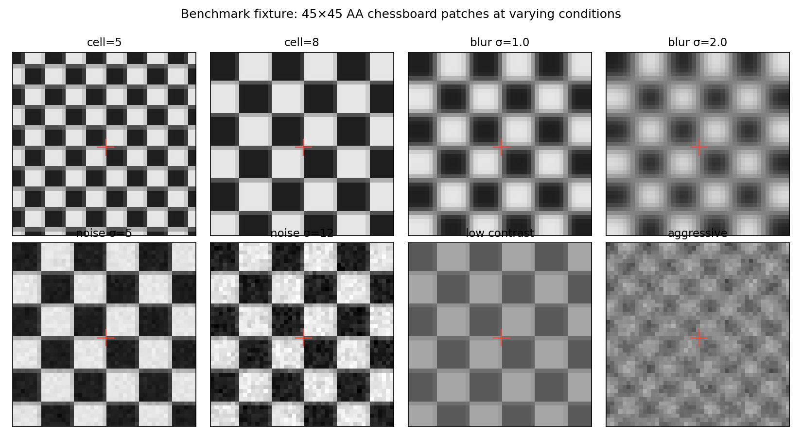
The red cross in each panel is the true corner. The 36 sub-pixel
offsets cover one full cell period, so each refiner sees the same
range of phase offsets within a cell. That is the only source of
within-condition variability on clean data — σ_noise = 0 means the
36 error values for a refiner at a given (cell, blur) setting are
fully deterministic. This matters for the CDF plot in §7.2.
This rendering mode is what we call “hard cells” elsewhere in this
book: sharp ink/paper step edges, softened by a Gaussian PSF, sampled
by pixels. It is what a camera produces when it images a printed
checkerboard. An alternative fixture common in machine-learning
papers uses a smooth saddle tanh(x)·tanh(y) model, which is easier
to differentiate analytically but has no sharp edges and does not
resemble sensor output.
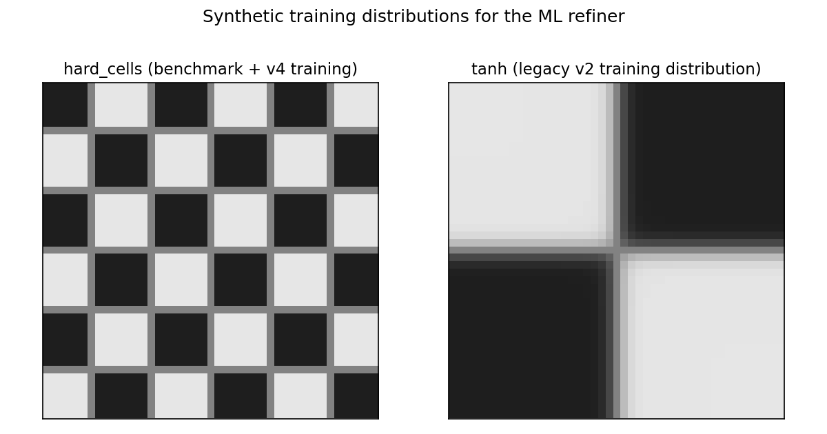
We use hard cells as the primary fixture. Part V §5.6.3 discusses
what happens when an ML refiner is trained on tanh data only.
7.2 Accuracy on clean cells
The figure below is the empirical CDF of Euclidean refinement errors
on the clean fixture (cell = 8 px, no blur, no noise). Each curve has
exactly 36 points — one per sub-pixel offset — so it rises in steps
of 1 / 36 ≈ 0.028. The stair pattern is not noise; it is the
empirical distribution of a deterministic 36-sample grid, the
standard way to draw an ECDF.
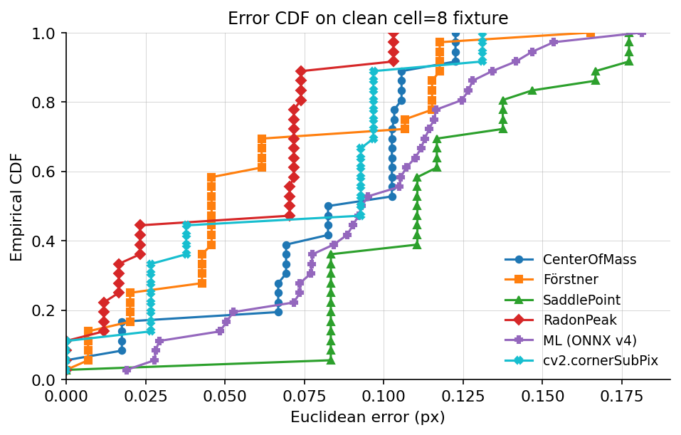
Reading the CDF:
- RadonPeak has the lowest errors across the whole distribution. Its 95th percentile sits below 0.12 px.
- Förstner and cv2.cornerSubPix cluster in the next band,
with mean around 0.06 px and
p95around 0.10 px. - CenterOfMass and ML (ONNX v4) land around 0.09 px mean /
0.15 px
p95. - SaddlePoint has a fat right tail on this fixture: its parabolic fit becomes ill-conditioned on a subset of the 36 offsets, and those outliers drag the mean up. With noise or blur added, the tail closes (see §7.3).
7.3 Accuracy vs blur
Log-y axis. The shaded band at 0.05–0.10 px marks the error range where a refiner is usable without per-scene tuning.
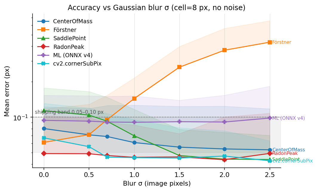
- Förstner is gradient-based. Gaussian smoothing flattens the
gradient magnitudes its structure tensor depends on, so its error
grows roughly linearly in
σ_blur. - Every other refiner stays inside the plotted 0.05–0.10 px band up to
σ_blur = 2.5 pxon this fixture. - RadonPeak and cv2.cornerSubPix have the lowest blur-row errors in this plot. Both integrate over neighborhoods that still contain useful signal after the step edge is smoothed.
The Radon detector is not shown on this plot because it is a detector, not a refiner. It uses the same response family as RadonPeak, but detector-level recall and precision are measured separately.
7.4 Accuracy vs additive noise
Log-y axis, same shaded band as §7.3.
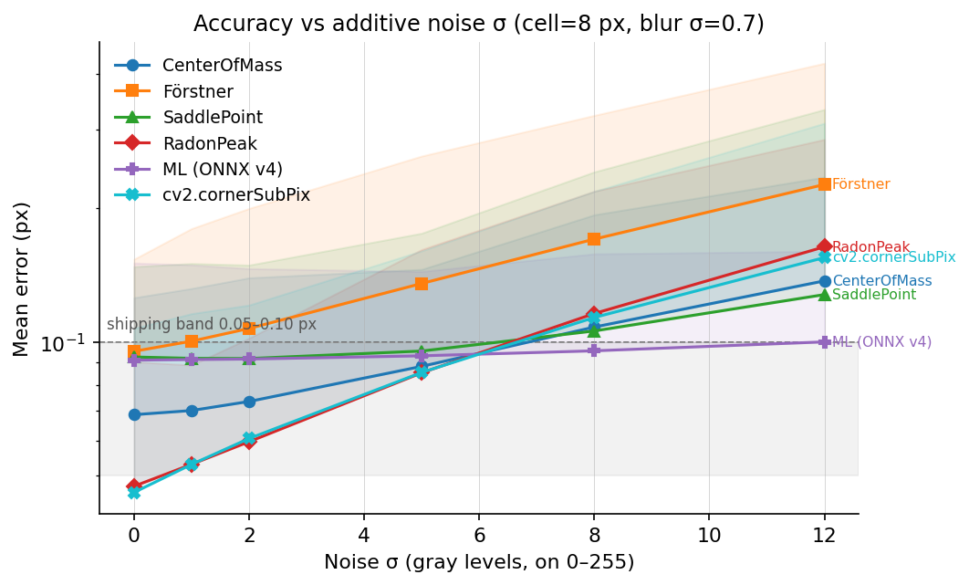
This is the regime where the ML refiner has the lowest mean error in
the plot. At σ_noise ≥ 8 gray levels, the ONNX v4 model is ahead of
the hand-coded methods on this synthetic fixture. The model was trained
with noise augmentation over σ ∈ [0, 10]; that is the strongest
supported explanation for the result here. Validate this separately on
real low-light frames before relying on it as a general rule.
7.5 Accuracy vs cell size
Largest operational plot. Two refiners break on small cells:
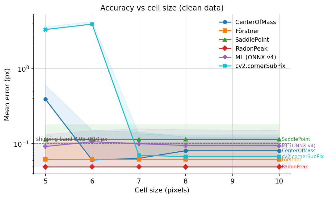
- cv2.cornerSubPix uses a default
winSize = (5, 5), which means an 11×11 search window. At cell size 5–6 px the window crosses into the two neighboring corners andcornerSubPixcollapses to around 3 px mean error. Passing a smallerwinSize(e.g.(2, 2)at cell = 5) fixes this, but the default is easy to overlook. - CenterOfMass uses the ChESS response ring at radius 5. At cell = 5 the ring crosses cell boundaries and the response-map centroid is biased by the neighbor corners, giving ~0.4 px mean error. At cell = 6 the crossover is minimal and the refiner recovers.
RadonPeak, Förstner, SaddlePoint, and ML look at a 2–3 px local neighborhood and are cell-size-agnostic down to 4 px. For dense targets (ChArUco, compact calibration boards) pick from those four.
7.6 Throughput vs accuracy
Log-log axes. Two orders of magnitude separate the fastest refiner (CenterOfMass at ~20 ns/corner) from ML inference (~250 µs/corner at batch = 1).
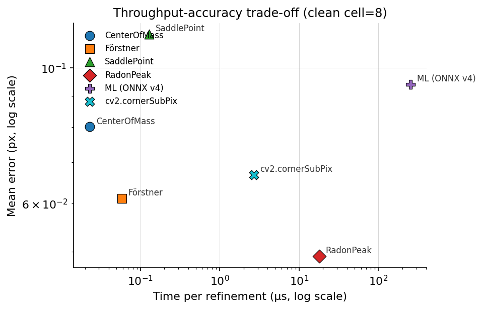
The Pareto frontier, fast-to-slow:
| Refiner | Time / corner | Clean-data mean error | Notes |
|---|---|---|---|
CenterOfMass | ~20 ns | 0.08 px | Unmatched throughput; fails at cell ≤ 5 (see §7.5). |
Förstner | ~60 ns | 0.06 px | Good on sharp images; degrades with blur. |
SaddlePoint | ~120 ns | 0.11 px | Stable across conditions; the no-surprise default. |
cv2.cornerSubPix | ~2.7 µs | 0.05 px | OpenCV’s refiner. Comparable accuracy to RadonPeak on clean data. |
RadonPeak | ~17 µs | 0.049 px | Lowest clean/blur error. ~140× SaddlePoint cost. |
ML (ONNX v4) | ~250 µs (b=1) | 0.09 px | Lowest error on the heaviest noise row in this fixture. |
The OpenCV timing in earlier revisions of this chapter was reported
at ~300 µs because the measurement loop included fixture construction;
the refinement-only value (~2.7 µs) is what the table above quotes.
See tools/book/opencv_subpix_sweep.py for the exact measurement
boundaries.
7.7 Whole-pipeline throughput
The per-refiner timings above are the refinement step alone. End-to-end detector-plus-refiner wall times on three test images, release build, averaged over 10 runs (milliseconds):
| Config | Features | small 720×540 | mid 1200×900 | large 2048×1536 |
|---|---|---|---|---|
| Single-scale | none | 3.01 | 4.46 | 26.02 |
| Single-scale | simd | 1.29 | 1.74 | 10.00 |
| Single-scale | rayon | 1.14 | 1.41 | 6.63 |
| Single-scale | simd+rayon | 0.92 | 1.15 | 5.34 |
| Multiscale (3 l) | none | 0.63 | 0.70 | 4.87 |
| Multiscale (3 l) | simd | 0.40 | 0.42 | 2.77 |
| Multiscale (3 l) | rayon | 0.48 | 0.52 | 1.94 |
| Multiscale (3 l) | simd+rayon | 0.49 | 0.54 | 1.59 |
Observations:
- Refinement dominates: the coarse detect stage takes 0.08–0.75 ms across these sizes; merge is a negligible fraction.
- Picking RadonPeak over SaddlePoint adds ~5–15 ms on a 1000-corner calibration frame. Usually acceptable for offline calibration, marginal for real-time loops.
- Picking ML at batch = 1 adds ~30 ms per 100 corners.
Feature flag guidance:
- Enable
simdwhen you are on nightly Rust and the target supports portable SIMD. It is the largest ChESS speedup in the table above. - Add
rayonfor images ≥ 1080p; on the small image in this benchmark, thread overhead can cancel the benefit. - Multiscale is the faster preset in this table. Use single-scale when you specifically want to compare against the full-resolution detector path.
7.7.1 Whole-image Radon detector
The Duda-Frese Radon path (DetectorConfig::radon()) is an alternative
detector for frames where ChESS’s 16-sample ring does not produce enough
seeds in the repository fixtures: heavy blur, low contrast, or small
cells. In this workload the Radon pipeline is several times slower than
the ChESS pipeline at the same resolution. For large frames,
DetectorConfig::radon_multiscale() can reduce cost by seeding on a
coarser level before refining in the input image.
Wall times on the same three test images, release build, averaged over 10 runs (milliseconds), 8-core M-class CPU:
| Stage | Features | small 720×540 | mid 1024×576 | large 2048×1536 | 1920×1080 synth |
|---|---|---|---|---|---|
| Response only | none | 130.6 | |||
| Response only | rayon | 27.9 | |||
| Response only | simd+rayon | 28.0 | |||
| Full pipeline | none | 28.6 | 31.3 | 298 | 162 |
| Full pipeline | rayon+simd | 28.8 | 19.6 | 188 | 162 |
End-to-end cumulative speedup vs. the scalar pre-opt reference (the state Radon shipped in at #45):
| Bench | Pre-opt | Post-opt (rayon+simd) | Speedup |
|---|---|---|---|
radon_response 1920×1080 up=2 | 130.6 ms | 28.0 ms | 4.7× |
radon_pipeline 1920×1080 synth | 692 ms | 162 ms | 4.3× |
radon_pipeline large.png | 393 ms | 188 ms | 2.1× |
radon_pipeline mid.png | 47 ms | 19.6 ms | 2.4× |
What was changed, in order:
- Row-parallel
compute_responseunderrayon, plus a handwrittenSimd<i64, 8>inner kernel undersimd. This is the biggest single win on the response stage (~4.7×). - Row-parallel
box_blur_inplaceunderrayon. The vertical pass was rewritten row-major (was column-strided), which also speeds up the scalar path 5–28% as a side effect. upsample_bilinear_2xandbuild_cumsumsparallelism — rayon row-wise on the upsampler,rayon::joinacross the four independent cumsum directions.merge_corners_simplespatial grid — the original O(N²) pairwise scan was the dominant cost on synthetic chessboards and low-contrast frames where Radon emits thousands of candidates. Replaced with a uniform spatial grid keyed on the merge radius (cell size =radius); expected O(N) for typical distributions. This is the single largest pipeline-level win (1920×1080 synth dropped from 665 ms to 185 ms with all features enabled).- Row-parallel NMS + peak-fit in
detect_peaks_from_radonunderrayon, with thread-local accumulators concatenated in row order to keep the output deterministic.
Caveats and notes:
- Portable SIMD on the inner kernel adds ~50% over scalar single-thread, but stacks weakly with rayon — the loop is memory-bound on M-class CPUs and rayon already saturates DRAM bandwidth. SIMD is the bigger relative win on AVX-512 hosts where the i64 lane width matches natively.
- The four cumsum directions remain individually serial (each has a
prefix-sum data dependency along its direction). Only the
inter-direction parallelism via
rayon::joinis added. - Small images (
small.pngat 720×540) fall outside the regime where rayon’s thread-startup overhead amortizes. The optimization mostly preserves their wall time rather than improving it.
The accuracy guard test
(crates/chess-corners/tests/perf_accuracy_guard.rs) locks down
recall, precision, and p95 subpixel error per detector mode so
optimization patches that change correctness fail at cargo test
rather than silently drifting in production.
7.8 Comparison with OpenCV
OpenCV ships two reference paths standard in calibration pipelines:
cv2.cornerSubPix— iterative gradient-based refiner, covered in §7.2–7.6 above as one of the refiner candidates.cv2.findChessboardCornersSB— a complete chessboard detector. Not a direct refiner comparison, but a useful reference for whole-pipeline accuracy on real calibration frames.
On the public Stereo Chessboard dataset (2 × 20 frames, 77 corners each):
- Pairwise distance,
findChessboardCornersSBvs our ChESS + default refiner: mean 0.21 px. - Pairwise distance,
cv2.cornerHarris + cornerSubPixvs ChESS: mean 0.24 px.
Neither reference is ground truth; both pipelines have their own sub-pixel biases on real imagery. The useful takeaway is that on real calibration frames the three methods agree to within about 0.25 px, consistent with the distributions in §7.2–7.5.
Wall-time, same dataset: findChessboardCornersSB takes ~115 ms
per frame; our detector takes ~4 ms per frame — a ~30× speedup.
7.9 Tracing and diagnostics
Build with the tracing feature to emit JSON spans for each pipeline
step. Named spans:
single_scale— single-scale path body.coarse_detect— response computation + candidate extraction.refine— per-seed refinement (carriesseedscount).merge— cross-level duplicate suppression.build_pyramid— pyramid construction.ml_refiner— ML path only; carries a batch-size event.radon_detect— Radon path only.
Capture traces via the CLI’s --json-trace flag or the
tools/perf_bench.py script. tools/trace/parser.py extracts spans
into CSV or JSON for aggregation, and tools/perf_bench.py produces
the table in §7.7.
When a frame returns fewer corners than expected:
- Check the
coarse_detectspan’s candidate count. If it is zero or very low, the detector failed to seed and no refinement ran. Consider switchingDetectorConfig::strategy(ChESS ↔ Radon) or lowering the threshold (cfg.threshold = Threshold::Relative(_)orThreshold::Absolute(_)). - If seeds are present but most
refineresults are rejected, the refiner’s thresholds are firing. Swap viaDetectorConfig.refiner.kindor relax the specific rejection (e.g. raiseSaddlePointConfig.max_offset). - If accuracy is fine but wall time is large, inspect the
refinespan. On the measured refiner benchmark, replacing RadonPeak / ML with a structure-tensor refiner is much cheaper per corner, with the accuracy tradeoff shown in §7.2–§7.6.
7.10 Integration recipes
Real-time loop, 30+ fps
#![allow(unused)]
fn main() {
use chess_corners::{ChessRefiner, Detector, DetectorConfig};

let cfg = DetectorConfig::chess_multiscale()
    .with_chess(|c| c.refiner = ChessRefiner::saddle_point());

let mut detector = Detector::new(cfg)?;

loop {
    let frame = next_frame();  // your camera source
    let corners = detector.detect(&frame)?;
    // ...
}
}
Detector reuses pyramid scratch buffers across frames; with
simd + rayon this stays under 2 ms on 1080p.
Offline calibration, maximum accuracy
#![allow(unused)]
fn main() {
use chess_corners::{Detector, DetectorConfig, RadonRefiner};

let cfg = DetectorConfig::radon_multiscale()
    .with_radon(|r| r.refiner = RadonRefiner::radon_peak())
    .with_merge_radius(2.0);

let mut detector = Detector::new(cfg)?;
let corners = detector.detect(&image)?;
}
The extra 5–15 ms per frame is invisible in an offline run.
Low-light / noise-heavy imagery
#![allow(unused)]
fn main() {
#[cfg(feature = "ml-refiner")]
{
use chess_corners::{ChessRefiner, Detector, DetectorConfig};

let cfg = DetectorConfig::chess_multiscale()
    .with_chess(|c| c.refiner = ChessRefiner::Ml);

let mut detector = Detector::new(cfg).unwrap();
let corners = detector.detect(&image).unwrap();
}
}
Requires the ml-refiner feature. The ML path batches candidates
internally; effective cost on a 100-corner frame is ~30 ms.
Small cells or heavy defocus — switch detector
#![allow(unused)]
fn main() {
use chess_corners::{DetectorConfig, Detector};

let cfg = DetectorConfig::radon();  // Radon detector with paper defaults
let mut detector = Detector::new(cfg)?;
let corners = detector.detect(&image)?;
}
In the synthetic sweeps, the Radon detector remains usable on smaller cells and heavier blur than the default ChESS ring (see Part IV §4.5).
Blurry / low-contrast imagery on large frames — Radon multiscale
#![allow(unused)]
fn main() {
use chess_corners::{DetectorConfig, Detector};

let cfg = DetectorConfig::radon_multiscale();
let mut detector = Detector::new(cfg)?;
let corners = detector.detect(&image)?;
}
Combines the Radon response kernel with the coarse-to-fine pyramid.
Prefer this over single-scale radon when the frame is ≥ 1280×960
and latency matters.
7.11 Reproducing every plot
# Cross-refiner accuracy sweep (Rust), feeds all Part VII plots
cargo run --release -p chess-corners --example bench_sweep \
    --features ml-refiner > book/src/img/bench/bench_sweep.json

# Same fixture, OpenCV cornerSubPix
python tools/book/opencv_subpix_sweep.py \
    --out book/src/img/bench/opencv_subpix_sweep.json

# Fixture panels (synth_grid.png, synth_modes.png)
python tools/book/synth_examples.py

# All accuracy + throughput plots
python tools/book/plot_benchmark.py

# Whole-pipeline timings on the three test images
python tools/perf_bench.py

# Integration test that gates refiner accuracy on CI
cargo test --release -p chess-corners --test refiner_benchmark \
    --features ml-refiner -- --nocapture --test-threads=1

# Recall / precision / p95-error guard against optimization regressions
cargo test --release -p chess-corners --test perf_accuracy_guard \
    --all-features

# Criterion benchmarks (default features = scalar reference)
cargo bench -p chess-corners        --bench radon_pipeline
cargo bench -p chess-corners        --bench chess_pipeline
cargo bench -p chess-corners-core   --bench refiners
cargo bench -p chess-corners-core   --bench radon_response

# Same benches under SIMD + rayon
cargo bench -p chess-corners        --bench radon_pipeline --features rayon,simd
cargo bench -p chess-corners-core   --bench radon_response --features rayon,simd

# Save a baseline before optimizing, then re-run with --baseline <name>
cargo bench --workspace -- --save-baseline pre-opt
cargo bench --workspace -- --baseline pre-opt

# Flamegraph / samply harness for hot-path profiling.
# Outputs under testdata/out/profiles/.
tools/profile.sh chess  testimages/large.png
tools/profile.sh radon  testimages/large.png
tools/profile.sh refiner saddle  testimages/mid.png
tools/profile.sh samply chess testimages/large.png
Part IX describes how to contribute code, tests, or datasets back to the project.
Part IX: Contributing
The workspace is a practical reference implementation rather than a one-off experiment. Contributions are welcome in three forms.
Bug reports and feature requests. Issues with reproduction steps and sample data are the most useful. Small synthetic fixtures that expose a failure mode are especially helpful because they can be added directly to the test suite.
Tests, benchmarks, and datasets. The Python helpers under tools/
and the images in testdata/ are designed for rerunning accuracy and
performance experiments after code changes. Extending them, or
contributing new datasets, is a good way to validate improvements.
The benchmark fixture in Part VIII §7.1
and the ML refiner pipeline in tools/ml_refiner/ have their own
knobs and regression gates.
Algorithms. ChESS and the Duda-Frese Radon detector are two
points in the design space. New detectors, refiners, or descriptor
variants can be added behind the same trait surfaces
(CornerRefiner, DetectorConfig presets, DenseDetector implementations) and benchmarked against the
shipped pipelines using crates/chess-corners/examples/bench_sweep.rs.
Proposals go in docs/, following the existing proposal-*.md
templates.
Pre-PR quality gates (also enforced in CI):
python3 tools/check_doc_versions.py
cargo fmt --all --check
cargo clippy --workspace --all-targets --all-features -- -D warnings
cargo test --workspace --all-features
cargo doc --workspace --no-deps --all-features
mdbook build book
See CLAUDE.md for the full set of workspace conventions, including
the layering rules between the core, facade, and pyramid crates.