Part VIII: Benchmarks and performance
This chapter measures what the library does on controlled synthetic fixtures and on real calibration frames. It covers the five refiners of Part V, the full detector pipeline with and without optional features, and a comparison against OpenCV’s corner pipeline. All plots are reproducible from the commands at the end of the chapter.
All absolute numbers are measured on a MacBook Pro M4 with a release build of the current tree. Hardware changes absolute timings. Treat the relative ordering as a property of these fixtures and this implementation, not as a promise for every camera dataset.
7.1 The benchmark fixture
Every accuracy plot in this chapter uses one synthetic fixture, kept
identical between crates/chess-corners/examples/bench_sweep.rs (Rust
refiners) and tools/book/opencv_subpix_sweep.py (OpenCV). For each
measurement condition:
- Render a 45×45 grayscale image of a periodic checkerboard with a
given cell size
cand a chosen true corner position(x₀, y₀). The renderer samples each output pixel at 8×8 sub-pixel positions inside the pixel footprint and averages the samples to produce the gray value. That anti-aliasing step is what lets the corner land at a continuous sub-pixel offset instead of being quantized to half-pixels by the rasterizer. - Apply a Gaussian blur of standard deviation
σ_blur. - Add independent Gaussian noise of standard deviation
σ_noiseto every pixel, seeded per offset for reproducibility. - Place the true corner
(x₀, y₀)on a 6×6 regular grid of sub-pixel offsets inside one cell — 36 offsets total per condition. - Seed each refiner at
round(x₀, y₀)so the starting error is at most ±0.5 px in each axis. Measure Euclidean distance from the refined position to the true corner.
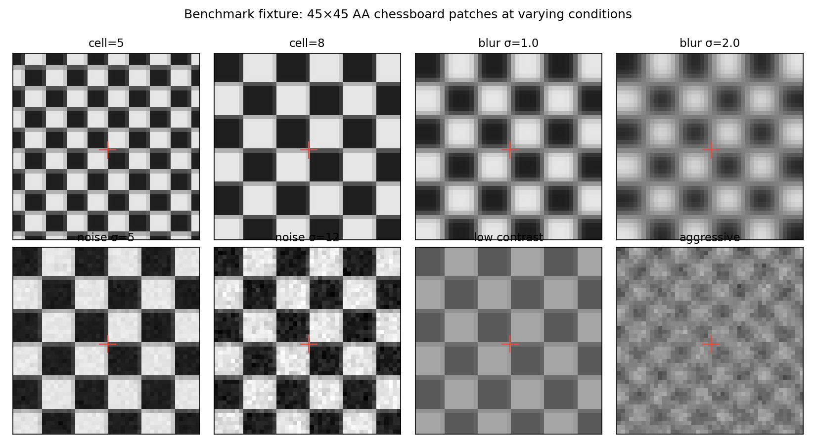
The red cross in each panel is the true corner. The 36 sub-pixel
offsets cover one full cell period, so each refiner sees the same
range of phase offsets within a cell. That is the only source of
within-condition variability on clean data — σ_noise = 0 means the
36 error values for a refiner at a given (cell, blur) setting are
fully deterministic. This matters for the CDF plot in §7.2.
This rendering mode is what we call “hard cells” elsewhere in this
book: sharp ink/paper step edges, softened by a Gaussian PSF, sampled
by pixels. It is what a camera produces when it images a printed
checkerboard. An alternative fixture common in machine-learning
papers uses a smooth saddle tanh(x)·tanh(y) model, which is easier
to differentiate analytically but has no sharp edges and does not
resemble sensor output.
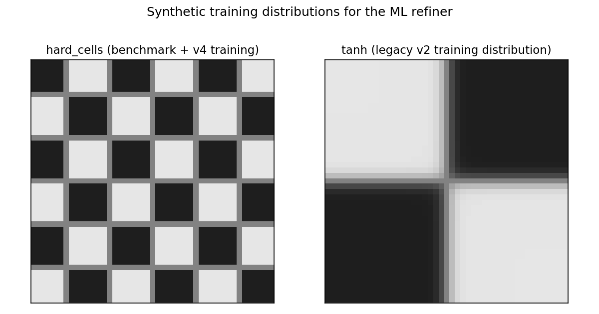
We use hard cells as the primary fixture. Part V §5.6.3 discusses
what happens when an ML refiner is trained on tanh data only.
7.2 Accuracy on clean cells
The figure below is the empirical CDF of Euclidean refinement errors
on the clean fixture (cell = 8 px, no blur, no noise). Each curve has
exactly 36 points — one per sub-pixel offset — so it rises in steps
of 1 / 36 ≈ 0.028. The stair pattern is not noise; it is the
empirical distribution of a deterministic 36-sample grid, the
standard way to draw an ECDF.
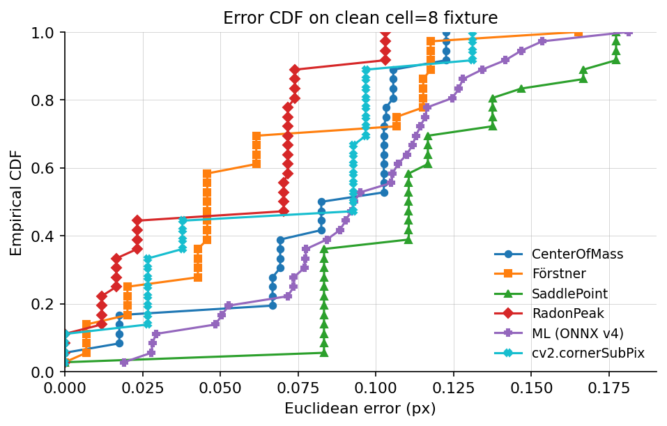
Reading the CDF:
- RadonPeak has the lowest errors across the whole distribution. Its 95th percentile sits below 0.12 px.
- Förstner and cv2.cornerSubPix cluster in the next band,
with mean around 0.06 px and
p95around 0.10 px. - CenterOfMass and ML (ONNX v4) land around 0.09 px mean /
0.15 px
p95. - SaddlePoint has a fat right tail on this fixture: its parabolic fit becomes ill-conditioned on a subset of the 36 offsets, and those outliers drag the mean up. With noise or blur added, the tail closes (see §7.3).
7.3 Accuracy vs blur
Log-y axis. The shaded band at 0.05–0.10 px marks the error range where a refiner is usable without per-scene tuning.
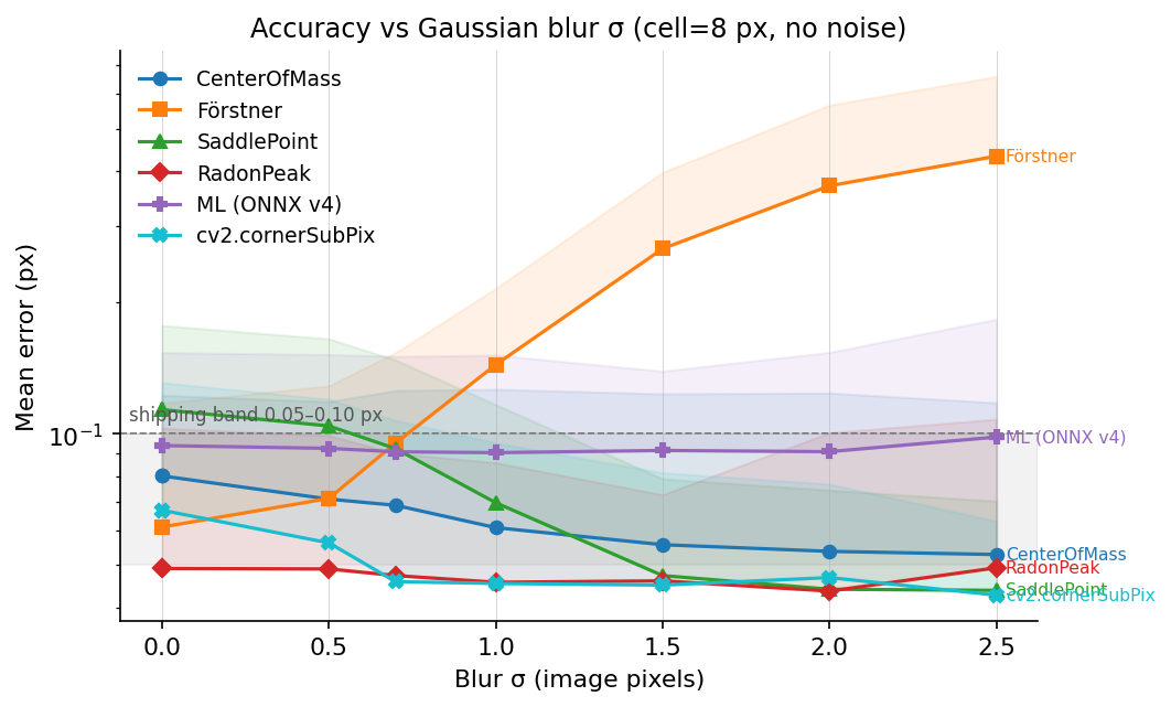
- Förstner is gradient-based. Gaussian smoothing flattens the
gradient magnitudes its structure tensor depends on, so its error
grows roughly linearly in
σ_blur. - Every other refiner stays inside the plotted 0.05–0.10 px band up to
σ_blur = 2.5 pxon this fixture. - RadonPeak and cv2.cornerSubPix have the lowest blur-row errors in this plot. Both integrate over neighborhoods that still contain useful signal after the step edge is smoothed.
The Radon detector is not shown on this plot because it is a detector, not a refiner. It uses the same response family as RadonPeak, but detector-level recall and precision are measured separately.
7.4 Accuracy vs additive noise
Log-y axis, same shaded band as §7.3.
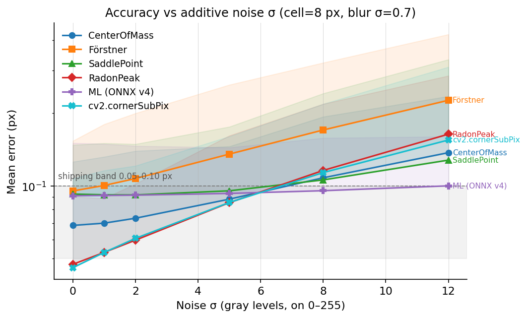
This is the regime where the ML refiner has the lowest mean error in
the plot. At σ_noise ≥ 8 gray levels, the ONNX v4 model is ahead of
the hand-coded methods on this synthetic fixture. The model was trained
with noise augmentation over σ ∈ [0, 10]; that is the strongest
supported explanation for the result here. Validate this separately on
real low-light frames before relying on it as a general rule.
7.5 Accuracy vs cell size
Largest operational plot. Two refiners break on small cells:
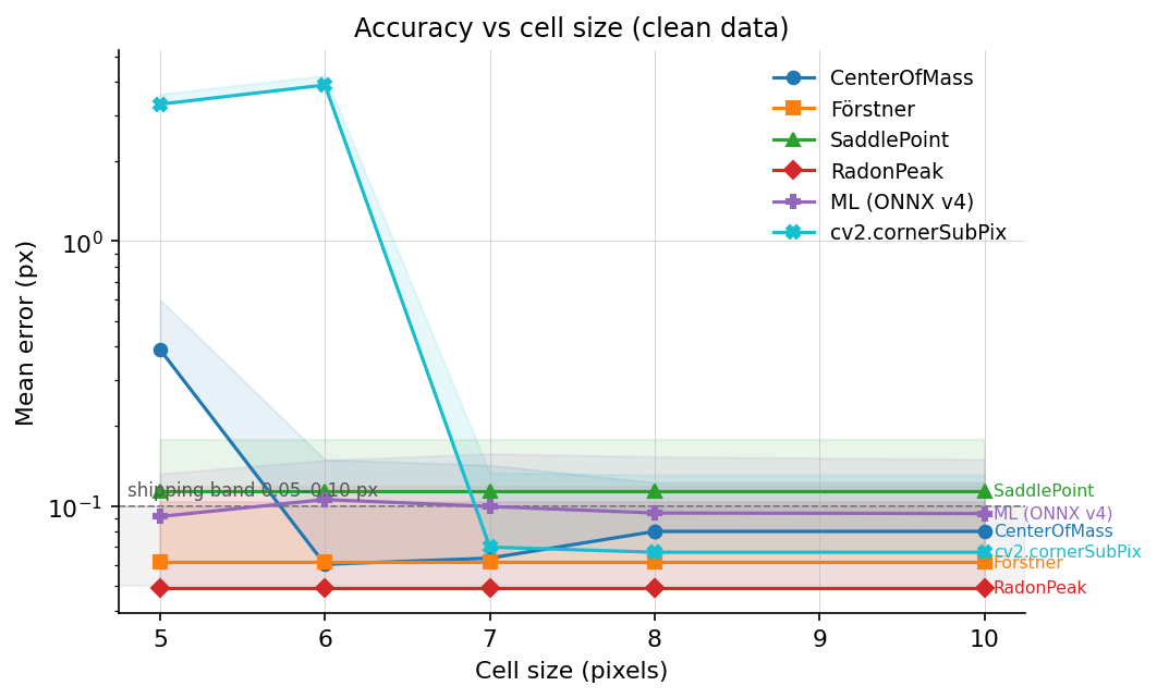
- cv2.cornerSubPix uses a default
winSize = (5, 5), which means an 11×11 search window. At cell size 5–6 px the window crosses into the two neighboring corners andcornerSubPixcollapses to around 3 px mean error. Passing a smallerwinSize(e.g.(2, 2)at cell = 5) fixes this, but the default is easy to overlook. - CenterOfMass uses the ChESS response ring at radius 5. At cell = 5 the ring crosses cell boundaries and the response-map centroid is biased by the neighbor corners, giving ~0.4 px mean error. At cell = 6 the crossover is minimal and the refiner recovers.
RadonPeak, Förstner, SaddlePoint, and ML look at a 2–3 px local neighborhood and are cell-size-agnostic down to 4 px. For dense targets (ChArUco, compact calibration boards) pick from those four.
7.6 Throughput vs accuracy
Log-log axes. Two orders of magnitude separate the fastest refiner (CenterOfMass at ~20 ns/corner) from ML inference (~250 µs/corner at batch = 1).
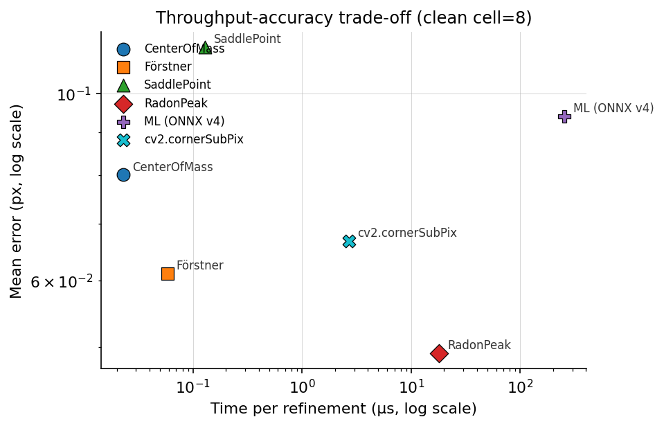
The Pareto frontier, fast-to-slow:
| Refiner | Time / corner | Clean-data mean error | Notes |
|---|---|---|---|
CenterOfMass | ~20 ns | 0.08 px | Unmatched throughput; fails at cell ≤ 5 (see §7.5). |
Förstner | ~60 ns | 0.06 px | Good on sharp images; degrades with blur. |
SaddlePoint | ~120 ns | 0.11 px | Stable across conditions; the no-surprise default. |
cv2.cornerSubPix | ~2.7 µs | 0.05 px | OpenCV’s refiner. Comparable accuracy to RadonPeak on clean data. |
RadonPeak | ~17 µs | 0.049 px | Lowest clean/blur error. ~140× SaddlePoint cost. |
ML (ONNX v4) | ~250 µs (b=1) | 0.09 px | Lowest error on the heaviest noise row in this fixture. |
The OpenCV timing in earlier revisions of this chapter was reported
at ~300 µs because the measurement loop included fixture construction;
the refinement-only value (~2.7 µs) is what the table above quotes.
See tools/book/opencv_subpix_sweep.py for the exact measurement
boundaries.
7.7 Whole-pipeline throughput
The per-refiner timings above are the refinement step alone. End-to-end detector-plus-refiner wall times on three test images, release build, averaged over 10 runs (milliseconds):
| Config | Features | small 720×540 | mid 1200×900 | large 2048×1536 |
|---|---|---|---|---|
| Single-scale | none | 3.01 | 4.46 | 26.02 |
| Single-scale | simd | 1.29 | 1.74 | 10.00 |
| Single-scale | rayon | 1.14 | 1.41 | 6.63 |
| Single-scale | simd+rayon | 0.92 | 1.15 | 5.34 |
| Multiscale (3 l) | none | 0.63 | 0.70 | 4.87 |
| Multiscale (3 l) | simd | 0.40 | 0.42 | 2.77 |
| Multiscale (3 l) | rayon | 0.48 | 0.52 | 1.94 |
| Multiscale (3 l) | simd+rayon | 0.49 | 0.54 | 1.59 |
Observations:
- Refinement dominates: the coarse detect stage takes 0.08–0.75 ms across these sizes; merge is a negligible fraction.
- Picking RadonPeak over SaddlePoint adds ~5–15 ms on a 1000-corner calibration frame. Usually acceptable for offline calibration, marginal for real-time loops.
- Picking ML at batch = 1 adds ~30 ms per 100 corners.
Feature flag guidance:
- Enable
simdwhen you are on nightly Rust and the target supports portable SIMD. It is the largest ChESS speedup in the table above. - Add
rayonfor images ≥ 1080p; on the small image in this benchmark, thread overhead can cancel the benefit. - Multiscale is the faster preset in this table. Use single-scale when you specifically want to compare against the full-resolution detector path.
7.7.1 Whole-image Radon detector
The Duda-Frese Radon path (DetectorConfig::radon()) is an alternative
detector for frames where ChESS’s 16-sample ring does not produce enough
seeds in the repository fixtures: heavy blur, low contrast, or small
cells. In this workload the Radon pipeline is several times slower than
the ChESS pipeline at the same resolution. For large frames,
DetectorConfig::radon_multiscale() can reduce cost by seeding on a
coarser level before refining in the input image.
Wall times on the same three test images, release build, averaged over 10 runs (milliseconds), 8-core M-class CPU:
| Stage | Features | small 720×540 | mid 1024×576 | large 2048×1536 | 1920×1080 synth |
|---|---|---|---|---|---|
| Response only | none | 130.6 | |||
| Response only | rayon | 27.9 | |||
| Response only | simd+rayon | 28.0 | |||
| Full pipeline | none | 28.6 | 31.3 | 298 | 162 |
| Full pipeline | rayon+simd | 28.8 | 19.6 | 188 | 162 |
End-to-end cumulative speedup vs. the scalar pre-opt reference (the state Radon shipped in at #45):
| Bench | Pre-opt | Post-opt (rayon+simd) | Speedup |
|---|---|---|---|
radon_response 1920×1080 up=2 | 130.6 ms | 28.0 ms | 4.7× |
radon_pipeline 1920×1080 synth | 692 ms | 162 ms | 4.3× |
radon_pipeline large.png | 393 ms | 188 ms | 2.1× |
radon_pipeline mid.png | 47 ms | 19.6 ms | 2.4× |
What was changed, in order:
- Row-parallel
compute_responseunderrayon, plus a handwrittenSimd<i64, 8>inner kernel undersimd. This is the biggest single win on the response stage (~4.7×). - Row-parallel
box_blur_inplaceunderrayon. The vertical pass was rewritten row-major (was column-strided), which also speeds up the scalar path 5–28% as a side effect. upsample_bilinear_2xandbuild_cumsumsparallelism — rayon row-wise on the upsampler,rayon::joinacross the four independent cumsum directions.merge_corners_simplespatial grid — the original O(N²) pairwise scan was the dominant cost on synthetic chessboards and low-contrast frames where Radon emits thousands of candidates. Replaced with a uniform spatial grid keyed on the merge radius (cell size =radius); expected O(N) for typical distributions. This is the single largest pipeline-level win (1920×1080 synth dropped from 665 ms to 185 ms with all features enabled).- Row-parallel NMS + peak-fit in
detect_peaks_from_radonunderrayon, with thread-local accumulators concatenated in row order to keep the output deterministic.
Caveats and notes:
- Portable SIMD on the inner kernel adds ~50% over scalar single-thread, but stacks weakly with rayon — the loop is memory-bound on M-class CPUs and rayon already saturates DRAM bandwidth. SIMD is the bigger relative win on AVX-512 hosts where the i64 lane width matches natively.
- The four cumsum directions remain individually serial (each has a
prefix-sum data dependency along its direction). Only the
inter-direction parallelism via
rayon::joinis added. - Small images (
small.pngat 720×540) fall outside the regime where rayon’s thread-startup overhead amortizes. The optimization mostly preserves their wall time rather than improving it.
The accuracy guard test
(crates/chess-corners/tests/perf_accuracy_guard.rs) locks down
recall, precision, and p95 subpixel error per detector mode so
optimization patches that change correctness fail at cargo test
rather than silently drifting in production.
7.8 Comparison with OpenCV
OpenCV ships two reference paths standard in calibration pipelines:
cv2.cornerSubPix— iterative gradient-based refiner, covered in §7.2–7.6 above as one of the refiner candidates.cv2.findChessboardCornersSB— a complete chessboard detector. Not a direct refiner comparison, but a useful reference for whole-pipeline accuracy on real calibration frames.
On the public Stereo Chessboard dataset (2 × 20 frames, 77 corners each):
- Pairwise distance,
findChessboardCornersSBvs our ChESS + default refiner: mean 0.21 px. - Pairwise distance,
cv2.cornerHarris + cornerSubPixvs ChESS: mean 0.24 px.
Neither reference is ground truth; both pipelines have their own sub-pixel biases on real imagery. The useful takeaway is that on real calibration frames the three methods agree to within about 0.25 px, consistent with the distributions in §7.2–7.5.
Wall-time, same dataset: findChessboardCornersSB takes ~115 ms
per frame; our detector takes ~4 ms per frame — a ~30× speedup.
7.9 Tracing and diagnostics
Build with the tracing feature to emit JSON spans for each pipeline
step. Named spans:
single_scale— single-scale path body.coarse_detect— response computation + candidate extraction.refine— per-seed refinement (carriesseedscount).merge— cross-level duplicate suppression.build_pyramid— pyramid construction.ml_refiner— ML path only; carries a batch-size event.radon_detect— Radon path only.
Capture traces via the CLI’s --json-trace flag or the
tools/perf_bench.py script. tools/trace/parser.py extracts spans
into CSV or JSON for aggregation, and tools/perf_bench.py produces
the table in §7.7.
When a frame returns fewer corners than expected:
- Check the
coarse_detectspan’s candidate count. If it is zero or very low, the detector failed to seed and no refinement ran. Consider switchingDetectorConfig::strategy(ChESS ↔ Radon) or lowering the threshold (cfg.threshold = Threshold::Relative(_)orThreshold::Absolute(_)). - If seeds are present but most
refineresults are rejected, the refiner’s thresholds are firing. Swap viaDetectorConfig.refiner.kindor relax the specific rejection (e.g. raiseSaddlePointConfig.max_offset). - If accuracy is fine but wall time is large, inspect the
refinespan. On the measured refiner benchmark, replacing RadonPeak / ML with a structure-tensor refiner is much cheaper per corner, with the accuracy tradeoff shown in §7.2–§7.6.
7.10 Integration recipes
Real-time loop, 30+ fps
#![allow(unused)]
fn main() {
use chess_corners::{ChessRefiner, Detector, DetectorConfig};

let cfg = DetectorConfig::chess_multiscale()
    .with_chess(|c| c.refiner = ChessRefiner::saddle_point());

let mut detector = Detector::new(cfg)?;

loop {
    let frame = next_frame();  // your camera source
    let corners = detector.detect(&frame)?;
    // ...
}
}
Detector reuses pyramid scratch buffers across frames; with
simd + rayon this stays under 2 ms on 1080p.
Offline calibration, maximum accuracy
#![allow(unused)]
fn main() {
use chess_corners::{Detector, DetectorConfig, RadonRefiner};

let cfg = DetectorConfig::radon_multiscale()
    .with_radon(|r| r.refiner = RadonRefiner::radon_peak())
    .with_merge_radius(2.0);

let mut detector = Detector::new(cfg)?;
let corners = detector.detect(&image)?;
}
The extra 5–15 ms per frame is invisible in an offline run.
Low-light / noise-heavy imagery
#![allow(unused)]
fn main() {
#[cfg(feature = "ml-refiner")]
{
use chess_corners::{ChessRefiner, Detector, DetectorConfig};

let cfg = DetectorConfig::chess_multiscale()
    .with_chess(|c| c.refiner = ChessRefiner::Ml);

let mut detector = Detector::new(cfg).unwrap();
let corners = detector.detect(&image).unwrap();
}
}
Requires the ml-refiner feature. The ML path batches candidates
internally; effective cost on a 100-corner frame is ~30 ms.
Small cells or heavy defocus — switch detector
#![allow(unused)]
fn main() {
use chess_corners::{DetectorConfig, Detector};

let cfg = DetectorConfig::radon();  // Radon detector with paper defaults
let mut detector = Detector::new(cfg)?;
let corners = detector.detect(&image)?;
}
In the synthetic sweeps, the Radon detector remains usable on smaller cells and heavier blur than the default ChESS ring (see Part IV §4.5).
Blurry / low-contrast imagery on large frames — Radon multiscale
#![allow(unused)]
fn main() {
use chess_corners::{DetectorConfig, Detector};

let cfg = DetectorConfig::radon_multiscale();
let mut detector = Detector::new(cfg)?;
let corners = detector.detect(&image)?;
}
Combines the Radon response kernel with the coarse-to-fine pyramid.
Prefer this over single-scale radon when the frame is ≥ 1280×960
and latency matters.
7.11 Reproducing every plot
# Cross-refiner accuracy sweep (Rust), feeds all Part VII plots
cargo run --release -p chess-corners --example bench_sweep \
    --features ml-refiner > book/src/img/bench/bench_sweep.json

# Same fixture, OpenCV cornerSubPix
python tools/book/opencv_subpix_sweep.py \
    --out book/src/img/bench/opencv_subpix_sweep.json

# Fixture panels (synth_grid.png, synth_modes.png)
python tools/book/synth_examples.py

# All accuracy + throughput plots
python tools/book/plot_benchmark.py

# Whole-pipeline timings on the three test images
python tools/perf_bench.py

# Integration test that gates refiner accuracy on CI
cargo test --release -p chess-corners --test refiner_benchmark \
    --features ml-refiner -- --nocapture --test-threads=1

# Recall / precision / p95-error guard against optimization regressions
cargo test --release -p chess-corners --test perf_accuracy_guard \
    --all-features

# Criterion benchmarks (default features = scalar reference)
cargo bench -p chess-corners        --bench radon_pipeline
cargo bench -p chess-corners        --bench chess_pipeline
cargo bench -p chess-corners-core   --bench refiners
cargo bench -p chess-corners-core   --bench radon_response

# Same benches under SIMD + rayon
cargo bench -p chess-corners        --bench radon_pipeline --features rayon,simd
cargo bench -p chess-corners-core   --bench radon_response --features rayon,simd

# Save a baseline before optimizing, then re-run with --baseline <name>
cargo bench --workspace -- --save-baseline pre-opt
cargo bench --workspace -- --baseline pre-opt

# Flamegraph / samply harness for hot-path profiling.
# Outputs under testdata/out/profiles/.
tools/profile.sh chess  testimages/large.png
tools/profile.sh radon  testimages/large.png
tools/profile.sh refiner saddle  testimages/mid.png
tools/profile.sh samply chess testimages/large.png
Part IX describes how to contribute code, tests, or datasets back to the project.