Part VI: Orientation methods

Both the ChESS detector and the Radon detector produce a list of corner candidates with subpixel positions. The descriptor pipeline lifts each position to a richer record that includes two grid-axis directions, their per-axis 1σ uncertainties, the corner contrast, and a fit residual. The “orientation method” is the algorithm that fits those axes from local image evidence — and because both detectors feed the same descriptor pipeline, the orientation method is detector-agnostic.

This chapter covers the two methods exposed by the public API, when to use each, and how each one works step by step.

6.1 API surface

The orientation_method field on DetectorConfig (and the OrientationMethod enum) selects which algorithm runs:

Both methods produce the same AxisFitResult shape: (theta1, theta2, sigma_theta1, sigma_theta2, amp, rms). They differ in the image evidence they use and in the failure modes they handle.

6.2 RingFit

RingFit samples 16 pixel values on a ring of radius \(r\) around the corner center and fits the parametric two-axis chessboard intensity model

\[ I(\varphi) = \mu + A \cdot \tanh\bigl(\beta \sin(\varphi - \theta_1)\bigr) \cdot \tanh\bigl(\beta \sin(\varphi - \theta_2)\bigr) \]

via Gauss-Newton, seeded from the 2nd-harmonic orientation of the ring samples. The slope \(\beta\) is fixed; the four free parameters are \(\mu, A, \theta_1, \theta_2\). Per-axis 1σ uncertainties are calibrated by a piecewise-linear LUT keyed on the contrast-relative residual, bringing reported sigmas closer to the empirical RMSE.

RingFit is suitable for the full range of standard chessboard images. It is the default and should be left in place unless you have a specific reason to switch.

6.3 When the ring fit isn’t enough

Three synthetic-patch cases motivate DiskFit and explain the lazy-gate logic. In each figure, ground truth is dashed white, the ring fit is red, and the disk fit is green.

Clean orthogonal corner

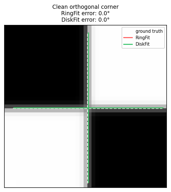
The 16-sample ring sits squarely on the four sectors of a canonical chessboard crossing. Both methods recover the axes within ~0.1°. The disk fit’s lazy gate detects this case from the ring’s contrast-relative residual (\(\text{rel_rms} < 0.04\)) and short-circuits to the ring fit, so you pay no extra cost on the easy corners.

Narrow projective skew

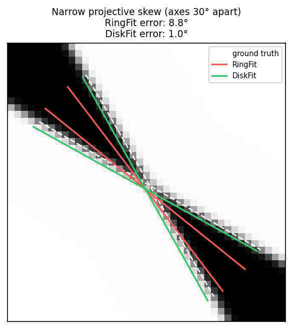
When projective warp pulls the two axes close together (here only 30° between them), the ring loses discriminative power: most ring samples sit in the two wide sectors and only a few sit in the narrow band between the lines. The 2nd-harmonic seed pulls the ring fit toward near-orthogonal axes, so it spreads the recovered angles outward (8.8° error). The disk fit looks at every pixel in the support disk — including the narrow-sector evidence the ring barely touches — and recovers both axes within 1°.

Sharp transition

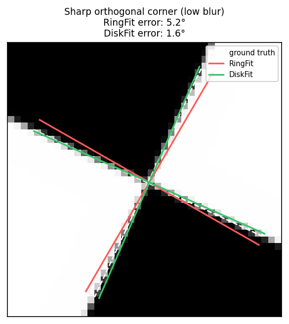
The ring fit’s parametric model fixes the tanh slope \(\beta = 4\), which matches a moderate edge width. On a sharp transition (\(w = 0.35\) px) the model cannot make its predicted intensity drop fast enough at the edge: the residual inflates and the angle estimate biases (5.2° error). The disk fit sweeps four widths \({0.35, 0.70, 1.40, 2.80}\) px and picks the one that minimises the relative residual, recovering both axes within 1.6°.

6.4 DiskFit, step by step

DiskFit models a corner as two crossing transition lines through the detected center. The intensity at every pixel \(p\) in a support disk around the center is fitted to

\[ I(p) = \mu + A \cdot \tanh!\Bigl(\frac{d_0(p)}{w}\Bigr) \cdot \tanh!\Bigl(\frac{d_1(p)}{w}\Bigr) \]

where \(d_0(p), d_1(p)\) are the signed perpendicular distances from \(p\) to the two lines and \(w\) is a discrete edge width drawn from \({0.35, 0.70, 1.40, 2.80}\) px. Recovering the corner means picking the line pair \((\theta_0, \theta_1)\) and width \(w\) that best reconstruct the disk’s pixel intensities.

The pipeline runs in seven steps:

1. Lazy-disk gate. If the ring fit’s relative residual rms / max(amp, 1) is below 0.04 and its axes are near-orthogonal (separation in [70°, 110°]), return the ring fit unchanged. Most chessboard corners pass this gate. The expensive disk pipeline only runs on suspect corners — extreme skew, blur, or low contrast — that fail one of these conditions.

2. Disk extraction. Sample a support disk of radius 1.6·r (capped at 8 px) around (cx, cy). Exclude the inner 1 px and any pixels outside the image. Require ≥ 64 valid pixels. For each pixel store its signed offset from the center, intensity, and 3×3 Sobel gradient (magnitude and direction).

3. Candidate generation. Build up to 64 candidate line directions from three sources, dropping any new candidate within 1°–4° of an existing one:

   • up to 8 peaks of a 72-bin gradient-direction histogram (smoothed with [0.25, 0.5, 0.25], pruned at 12% of the dominant peak);
   • both ring-fit seed angles ± {0°, 4°, 8°};
   • a coarse 30°-spaced global grid as a deterministic safety net.

   Histogram peaks find the truly observable lines; seed offsets cover the easy case; the global grid catches degenerate gradient distributions.

4. Pair pruning. Form all candidate pairs whose angular separation lies in [12°, 89.5°]. Score each pair by Gaussian-weighted per-pixel gradient alignment (σ = 4° around each candidate angle). Keep the top 24 by score; force-include the pair closest to the ring-fit seed and the pair of the two strongest single-candidate alignments so high-evidence seeds are never dropped.

5. Closed-form fit per pair × width. For each surviving pair and each width, compute q_p = tanh(d₀_p/w) · tanh(d₁_p/w) for every disk pixel and solve the OLS regression I_p − μ̂ ≈ A · q_p for amplitude A directly from sufficient statistics. The residual SSR falls out of the same statistics — no second pass over the disk. The objective is rel_rms − 1.25·edge_score, with \( \text{rel_rms} = \mathrm{rms} / \max(|A|, 1) \). Keep the top 2 fits by deterministic comparator (objective, then rel_rms, then edge_score, then narrower w, then smaller angles).

6. Local refinement. Around each top-2 seed, grid-search angle perturbations at step sizes {1°, 0.5°, 0.25°} (3×3 grid per step, 24 trials per seed). Width is held fixed.

7. Acceptance. Replace the ring fit only when the disk fit clears minimum amplitude (A ≥ 10), correlation (≥ 0.74), and edge support (≥ 0.035), AND one of:

   • rel_rms beats the ring fit by absolute margin (≥ 0.03) or ratio (≤ 92%);
   • axis separation is strongly non-orthogonal (< 55°);
   • axis separation is ≥ 75° AND w ≤ 0.7 px (sharp orthogonal);
   • the disk axes disagree with the ring axes by > 12° and edge support is ≥ 0.18.

   When accepted, the per-axis sigma is recomputed from the recovered separation and rel_rms (a 1.5°/3° floor depending on whether separation is ≥ 55° or not, plus 8·rel_rms capped at 6°, all scaled by 0.55). When rejected but the disk and ring axes disagreed by more than 12°, the ring fit’s sigma is inflated to at least 10° to flag the ambiguity.

6.5 Choosing a method

DiskFit costs more per corner than RingFit in the orientation benchmark (~131 µs vs ~15 µs for the measured case), but the lazy gate short-circuits clean orthogonal inputs. Switch to DiskFit when working with images that have known projective warp; otherwise leave the default in place.

For the per-method precision/cost trade-off on the synthetic bench, see the orientation bench REPORT.md in tools/orientation_bench/. The patch overlays in §6.3 are reproducible via tools/render_orientation_overlays.py.

Next: Part VII covers the multiscale pipeline that drives the detector across a Gaussian pyramid.